Support Vector Machines
Overview
Support Vector Machines (SVMs) are a powerful class of machine learning algorithms used for classification and regression tasks. They are particularly renowned for their effectiveness in separating data into distinct classes. “The main idea is that based on the labeled data (training data) the algorithm tries to find the optimal hyperplane which can be used to classify new data points. In two dimensions the hyperplane is a simple line”.1 In this overview, we will delve into the fundamentals of SVMs, exploring why they are adept at linear separation and how kernel functions play a pivotal role in their success. Furthermore, we will examine the criticality of dot products in SVMs and take a closer look at two essential kernel functions: the polynomial kernel and the radial basis function (RBF) kernel.
Introduction to Vectors
As one may assume from the name of this machine learning technique, SVMs use the mathematical concept of vectors and vector spaces to linearly separate numerical data into classes that can be then use to classified unlabeled data.
The simplest example of a vector can be thought of as a directional arrow to a point on a 2-dimensional coordinate plane.
Here the horizontal axis is associated with the variable “x” and the vertical axis is associated with the variable “y”. Then we can plot the instance that x=1 and y=2 as a point in the graph, but a vector gives more information as it has length and direction as seen by the blue arrow.
In the example, the tail of the vector is at the origin (0,0) and the tip is at the point in space (1, 2). Points and vectors are different but similar. Points are just a position in the coordinate system (like the black dots).
Thinking about vectors in the eyes of computer science one can think of them as “ordered lists of numbers”.2 For example, one can portray the test scores of a student in the order “GPA”, “Exam1”, and “Exam2” as [3.95, 100, 85], which is a vector. Consistent order matters! SVMs uses both of the interpretations together to create a supervised learning model for quantitative data.
Linear Separation and Support Vector Machines
At their core, Support Vector Machines are designed to find the optimal linear separation between different classes of data points. This linear separator is then used to identify the appropriate classification of new data vector points. When choosing a linear separator or separating hyperplane (in the cases of more than 2 dimensions), there are infinite possibilities that satisfy separating the training data, but not all of them are optimal for classifying new data vectors. For finding the optimal separator one aims to maximize the margin (the space between the separating hyperplane and the nearest data points of each class), known as support vectors. What makes SVMs especially effective at handling both linearly and non-linearly separable data is the use of higher dimensionalities with kernels.
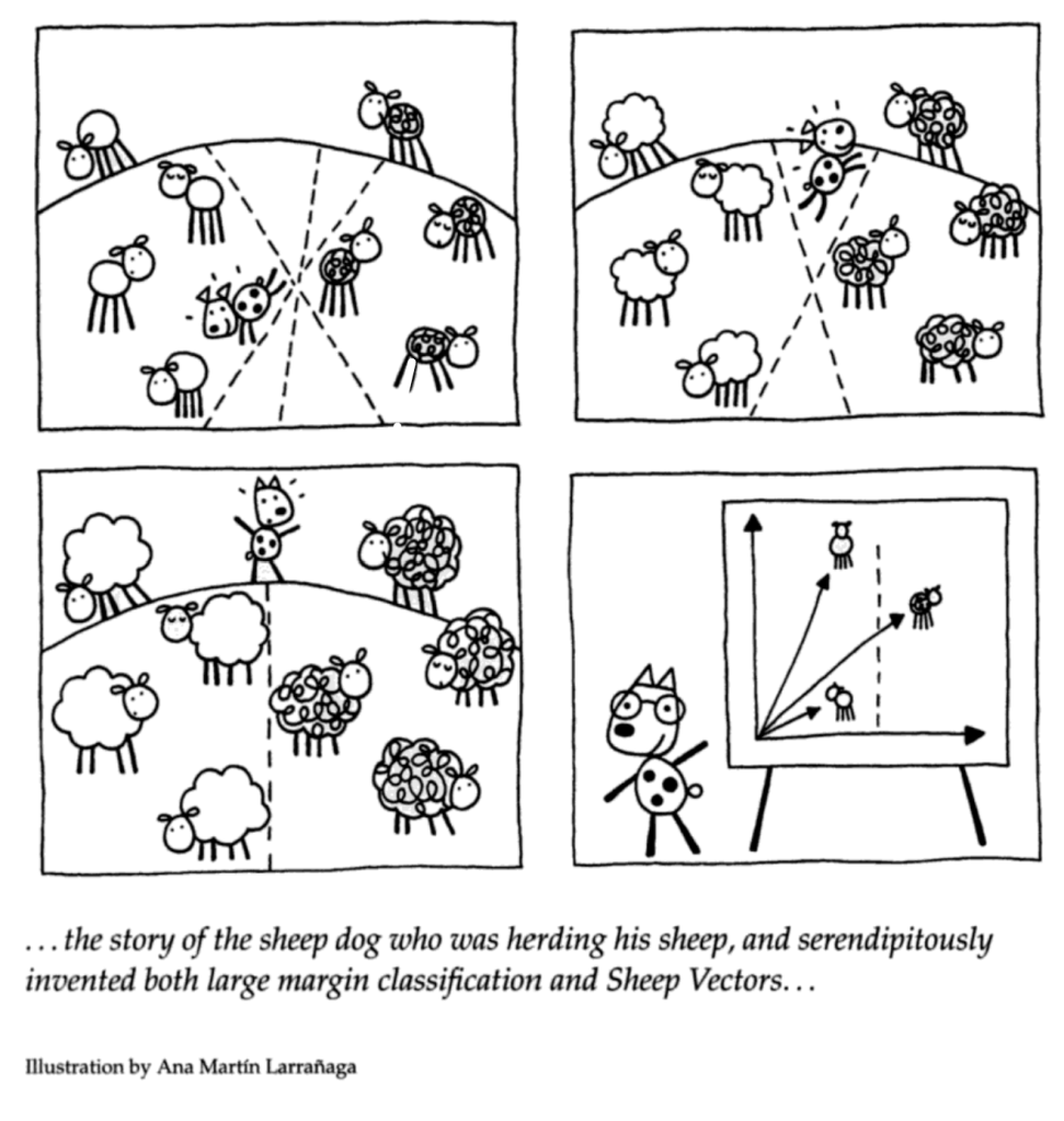
In the illustration the dog is able to make a linear separator between the different kinds of sheep. The dog has lots of different options for how to separate the sheep. But by “maximizing the margin” the dog is able to find a simple separator that will allow for more sheep as they age to remain separated. The sheep example is a two dimensional case, as the vectors are the 2-dimensional locational points of where the sheep are located on the field. The kinds of sheep are the different classes, or labels.
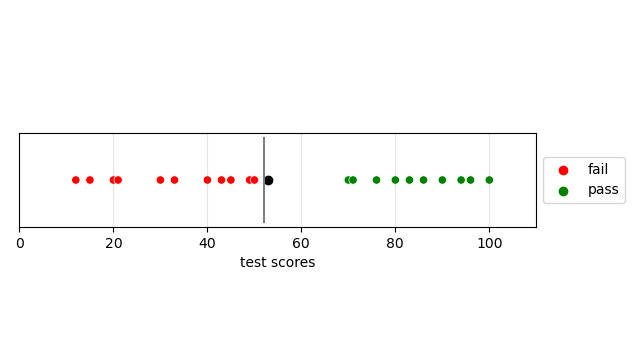
Let’s first look at this linear separation in a the simplest case, 1-dimensions. Suppose we have the classification problem of passing and failing test scores. In the graph we have all points in red as classified as failing and all green points classified as passing. Then we can set a threshold with the line. Suppose we are given a new test score of 35, then since it is less than the determined threshold it will be classified as failing.
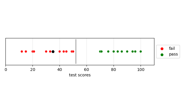
One issue with our choice of linear separation is that the distance from the current maximum failing score to the grey line is smaller than the distance of the current minimum passing score to the grey line. Which means, if this was a SVM model then some future values might be misclassified.
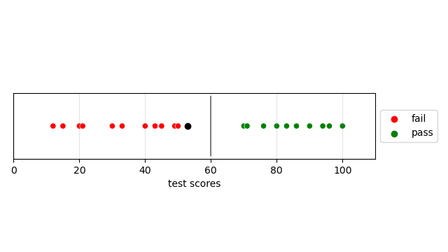
Suppose we get a new test score value of 56, our model now looks like this. Given the new data as shown by the black dot, we can see that 56 looks more grouped with the “fail” values, but because the separator is less than the new point, it will be classified as “pass”. This goes against our intuition as their appears to be two distinct clusters and 56 is closer to the “fail” cluster.
Now let’s suppose the threshold that is placed in the midpoint from the two clusters edges. This would be a better spot for classifying future data, as seen in the graph. This distance from the separator represented by the grey line and the nearest datapoint is called the margin. When the threshold is placed in the midpoint of the two clusters the margin is maximized. By maximizing the margin it allows for new data on the boundaries of clusters to still be associated with the closest cluster.
Reminder, when training a model we are given the training data and the labels (if it is supervised), we are NOT given a predetermined threshold value. If a predetermined threshold value is known, then a supervised learning model only adds uncertainty to a certain system.
Maximizing the margin in Support Vector Machines (SVMs) is advantageous for several reasons:
- Improved Generalization: A larger margin often leads to better generalization performance. The margin represents the separation between different classes, and a wider margin implies a clearer distinction between classes. This helps the SVM perform well on new, unseen data, reducing the risk of overfitting to the training data.
- Increased Robustness to Noise: A wider margin acts as a buffer against noise and outliers in the data. By focusing on the instances near the decision boundary, SVMs are less likely to be influenced by noisy data points that may not represent the true characteristics of the classes.
- Enhanced Resistance to Overfitting: SVMs with a larger margin are less susceptible to overfitting. Overfitting occurs when a model captures noise or fluctuations in the training data that do not reflect the underlying patterns in the data. Maximizing the margin helps to ensure that the model generalizes well to new data.
- Clear Decision Boundary: maximum-margin hyperplane provides a clear decision boundary between classes. This makes the classification process more intuitive and easier to interpret. Additionally, a well-defined decision boundary contributes to the model’s robustness and stability.
- Facilitation of Out-of-Sample Predictions: The wide margin allows for a greater tolerance for errors and variations in the input data, making SVMs effective in handling out-of-sample predictions. This is crucial in real-world scenarios where the distribution of data may change over time.
- Optimal Trade-off in Non-linear Classifications: In the case of non-linearly separable data, maximizing the margin contributes to finding a balance between fitting the training data well and maintaining a generalizable model. Techniques like the kernel trick enable SVMs to achieve this optimal trade-off.
In summary, maximizing the margin in SVMs enhances the model’s generalization, robustness, and resistance to overfitting, making it a powerful tool for various classification tasks, especially in scenarios with complex and high-dimensional data.
Kernel Functions
The power of SVMs extends beyond classic linear separation through the use of kernel functions. Kernels enable SVMs to transform data into higher-dimensional spaces, making it easier to find separating hyperplanes when linear separation is not feasible in the original feature space. “The Kernel Trick” empowers the SVM to operate without requiring knowledge of the precise mapping of each point within the nonlinear transformation. Instead, it focuses on understanding the relative relationships between data points after the nonlinear transformation has been applied.3 “Kernel functions only calculate the relationships between each pairs of points as if they are in the higher dimensions; they do not actually transform the data”4.
The Significance of Dot Products
To understand the role of kernel functions, it’s essential to comprehend the significance of dot products and what they are in general.

Now math can feel like a religion or even magic in some cases. In the case of math, it is a magic that one can learn the spells and harness its power if the foundations are strong and true. The techniques developed in linear algebra transcend many topics outside of just pure mathematics, the dot product is one of these amazing mathematical techniques that finds its way into many many topics. So what is the dot product?
Coordinate Definition
The dot product of two vectors a and b, where a and b are defined as such
![\mathbf{a} = [a_1, a_2, ... , a_n]](https://s0.wp.com/latex.php?latex=%5Cmathbf%7Ba%7D+%3D+%5Ba_1%2C+a_2%2C+...+%2C+a_n%5D&bg=ffffff&fg=000&s=0&c=20201002)
![\mathbf{b} = [b_1, b_2, ... , b_n]](https://s0.wp.com/latex.php?latex=%5Cmathbf%7Bb%7D+%3D+%5Bb_1%2C+b_2%2C+...+%2C+b_n%5D&bg=ffffff&fg=000&s=0&c=20201002)
then the dot product of vectors a and b can be defined as following

Here we can think of it as the vectors multiply pairs of numbers and then add them. Another way of defining the dot product is with the geometric definition. If the vectors are defined as column vectors then the dot product can be written as the matrix multiplication as such
![\mathbf{a} \cdot \mathbf{b} = \mathbf{a}^{T}\mathbf{b} = [a_1, a_2, ... , a_n]\begin{bmatrix}b_1\\ b_2\\ .\\.\\.\\ b_n\\ \end{bmatrix} = a_1b_1 + a_2b_2 + ... + a_nb_n](https://s0.wp.com/latex.php?latex=%5Cmathbf%7Ba%7D+%5Ccdot+%5Cmathbf%7Bb%7D+%3D+%5Cmathbf%7Ba%7D%5E%7BT%7D%5Cmathbf%7Bb%7D+%3D+%5Ba_1%2C+a_2%2C+...+%2C+a_n%5D%5Cbegin%7Bbmatrix%7Db_1%5C%5C+b_2%5C%5C+.%5C%5C.%5C%5C.%5C%5C+b_n%5C%5C+%5Cend%7Bbmatrix%7D+%3D+a_1b_1+%2B+a_2b_2+%2B+...+%2B+a_nb_n&bg=ffffff&fg=000&s=0&c=20201002)
Geometric Definition
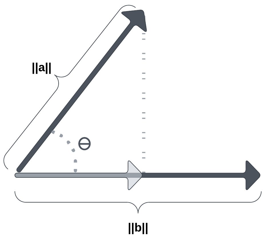
The dot product of two Euclidean vectors a and b is defined by

where 
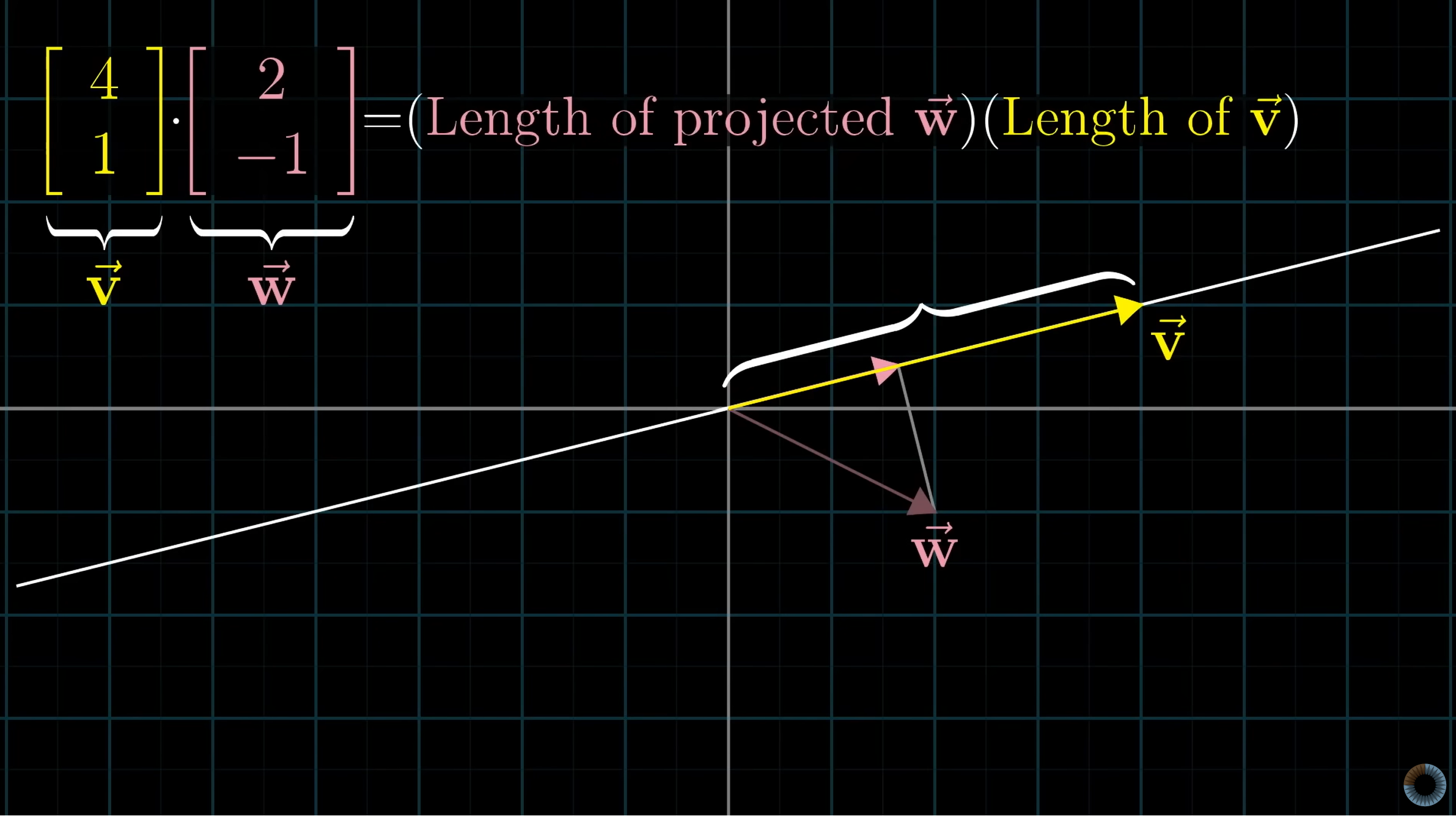
Let’s say we have two vectors v and w, then we can geographically understand the dot product to be the magnitude of vector v times the magnitude of vector w times the cosine of the angle between the two vectors.
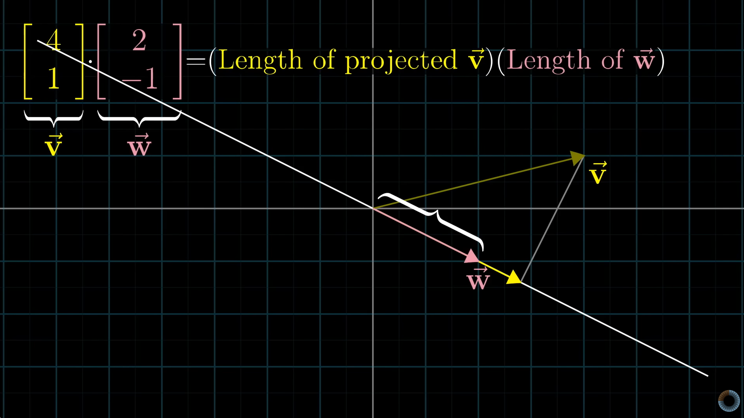
Another way of interpreting the dot product geographically is the magnitude of the scalar projection of v onto w multiplied by the magnitude of the vector w. Due to duality this is the same as magnitude of the scalar projection of w onto v multiplied by the magnitude of the vector v.
For a deeper understanding of duality and dot products check out the video “Dot products and duality | Chapter 9, Essence of linear algebra” by the YouTube channel Three Blue One Brown.
All three of these interpretations are equal by the definition of projections and the commutative property of multiplication of scalars.
Given vectors a and b then the projection of a onto b is

Where
Thus,

and

Important Note: Since 
Kernel and the Dot Product
In the case of non-linearly separable data, SVMs can use kernel functions to implicitly map the input vectors into a higher-dimensional space where they become linearly separable. The dot product is still at the core of this process, as the kernel function computes the dot product between the mapped vectors in the higher-dimensional space. The kernel function, takes as input two points in the original space, and directly gives us the dot product in the projected space. Popular kernel functions include the polynomial kernel and the radial basis function (RBF) kernel.
Polynomial and RBF Kernel Functions
Two common kernel functions in SVMs are the polynomial kernel and the radial basis function (RBF) kernel. Kernels “allow us to do linear discriminants on nonlinear manifolds, which can lead to higher accuracies and robustness than traditional linear models alone”. 5 The kernel function is just a mathematical function that transforms an input space into a higher-dimensional space. After this transformation the data become linearly separable, which then means one can use vector algebra and a support vector machine can be used to find a hyperplane that separates the data. By using kernels, SVMs will also have less errors as one can linearly separate data that previously was not in a lower dimension.
The Polynomial Kernel
In a nutshell, the polynomial kernel considers the original features of our dataset, much like the linear kernel. However, it goes a step further by taking into account the interactions between these features.6 The Polynomial Kernel, like all SVM kernels, systematically find Support Vector Classifiers (find the hyperplane that maximizes the margin between classes while minimizing classification errors) in higher dimensions.7
An important component of the polynomial kernel is its parameter d, which stands for the degree of the polynomial. The polynomial kernel then computes the d-dimensional relationships between each pair of the points to find the SVC. Thus, let’s define the polynomial kernel as follows

where a and b are vectors, r is the coefficient of the polynomial, and d is the degree of the polynomial. To figure out what the coefficient r and degree d should be it is recommended to perform cross validation and try out different values.
The RBF Kernel
The RBF kernel finds Support Vector Classifiers in infinite dimensions. How the Radial Basis Function Kernel works is familiar to that of the Nearest Neighbors algorithm and therefore new observations are strongly influenced by the closest observations for how it is classified, and further away observations have relatively low influence on the classification of these new observations. Thus, let’s define the RBF kernel as follows

where 

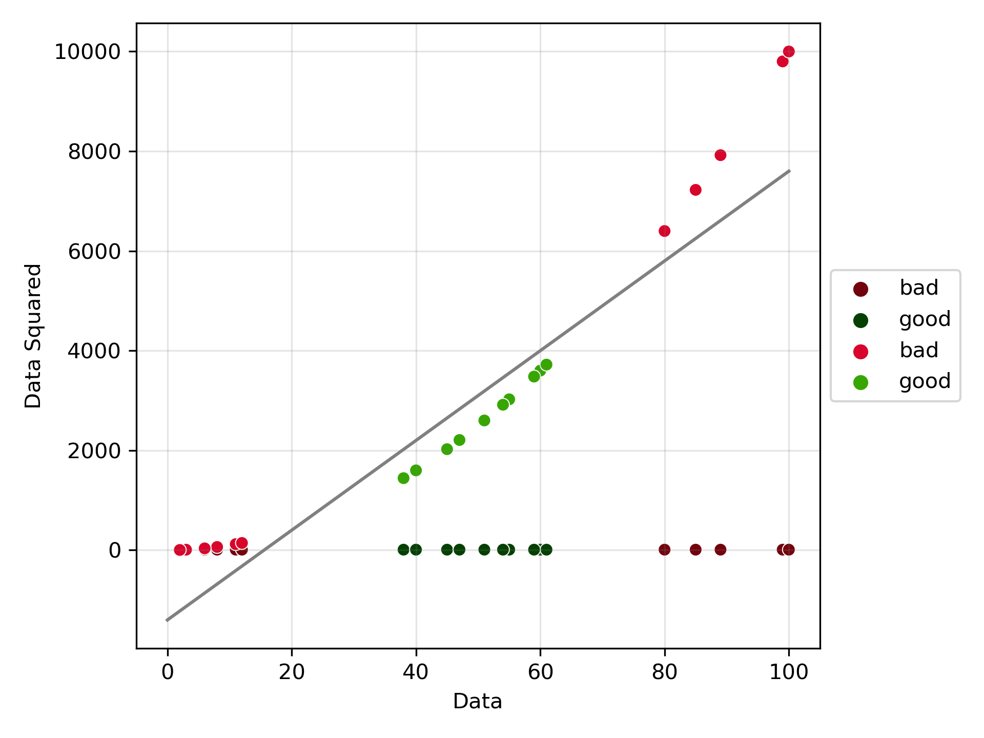
Example: Transforming a 2D Point with a Polynomial Kernel
As seen in the 1-D test score example above, we were able to find a linear separator that would effectively separate the failing from passing test scores. Now let’s Look at an example where that is not as easily achieved.
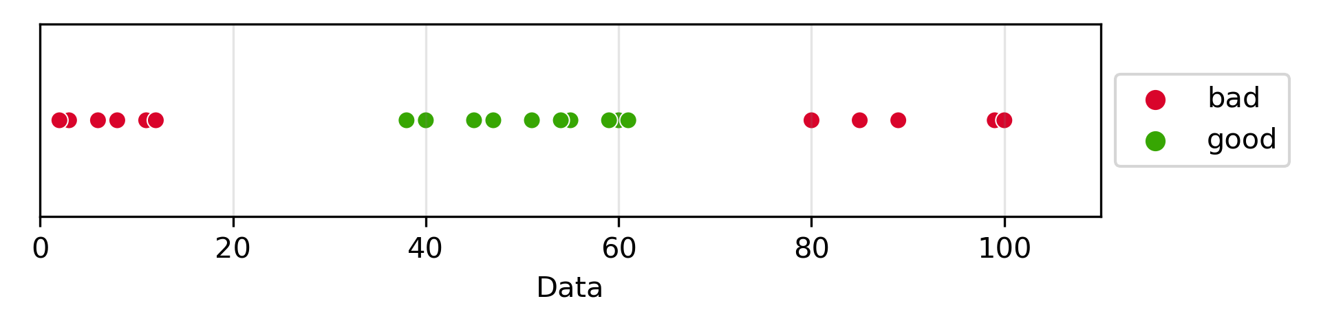
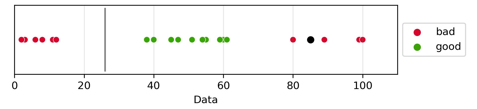
Let’s say we have the following problem. We have data that fits to two labels, “good” and “bad”. This good is for the data that is in middle range, the researchers desired that the data found in the higher ranges are “bad” for multiple reasons. Now, supposed we are given new data and would like to label it as “good” or “bad”.
Looking at the 1-dimensional data there is no linear separator in its current state that can separate the “good” and the “bad”. For example if we place the linear separator to the left of the good, we would misclassify a new high level point as “good”. However, if we place the separator to the right of the “good”, then future low values would be identified as “good” even though we can see it is more appropriately identified as “bad”.
In this case, let’s try implementing a polynomial kernel of degree 2. As seen in the graph, the data is now “transformed” to 2-dimensions. Note, that in the kernel trick the data is not actually transformed, only that the dot product allows for classification in this higher dimensional space.
Now we can easily place a linear separator between the labeled classes of “good” and “bad”, and identify new data points in the future with better accuracy.

Thus, Support Vector Machines, with their ability to perform linear separation and use the power of kernel functions, are incredible tools in machine learning. Understanding their operation, the role of dot products, and the application of kernel functions is key to successful utilization. Moving forward with all of this in mind, let’s perform SVM on wildfire data in the United States for year 2000 to 2022, with the aim of gaining further insights into this devastating natural disaster.
Data Prep
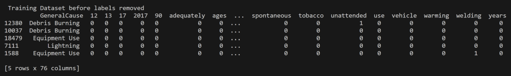
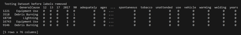
For the analysis of Wildfires in the United States from 2000 to 2022, the support vector machine modeling was performed on multiple datasets each with different purposes of them. These include quantitative values for the Acres Burned identifying the time of year the fire took place, to that of predicting the topic of an article based on the words used its headline. In order to perform supervised learning appropriately each of the datasets were split into disjoint training and testing datasets with their labels removed (but kept for reference and accuracy analysis). In supervised learning, labels are essential for two primary reasons. They provide the correct output for a given input, allowing the algorithm to learn and make predictions. Labels also enable model evaluation and performance assessment, serving as the basis for key metrics.
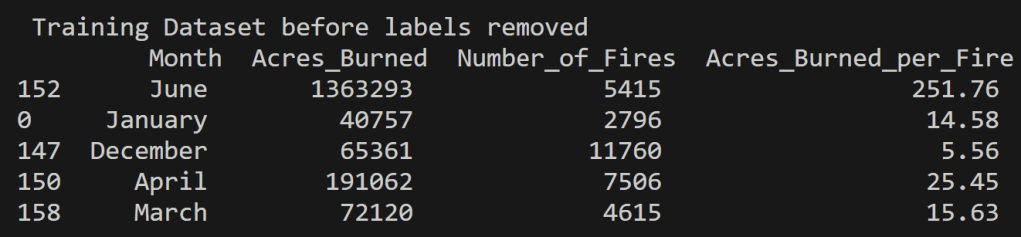
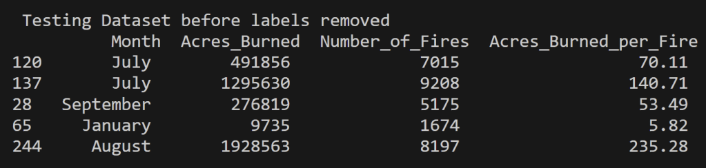
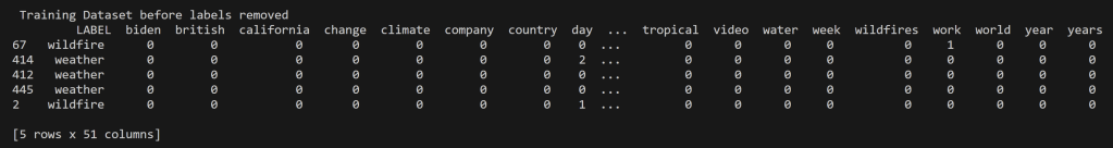
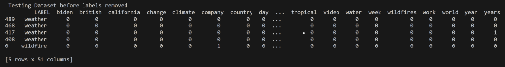
Below is the training and testing datasets that used a random split to have 80% of the data for training and 20% for testing. The goal for a good training set is for all of the possible data values to be represented and be represented in a proportion such that overfitting/underfitting for particular values doesn’t occur. All cleaned data used in this analysis can be found in the project GitHub repository here. Note that the datasets below have the labels still attached for reference, but they were removed from the testing set when running the predictions using the SVM model.
US Wildfires By Season for Years 2000 to 2022
News Headlines from September 16th, 2023
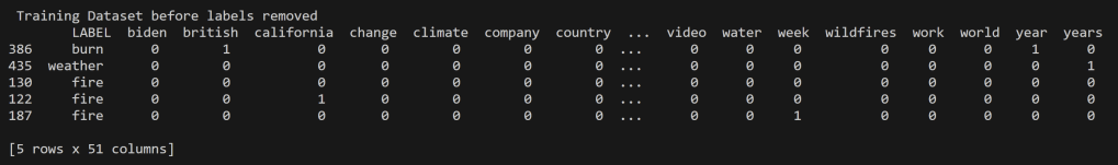
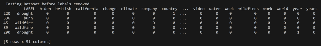
News Headlines for topics “wildfire” and “weather” from September 16th, 2023
Oregon Weather and Wildfires Cause Comments Years 2000 to 2022
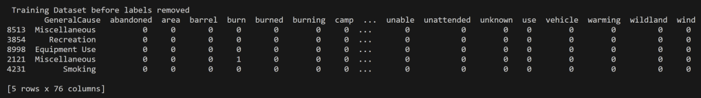
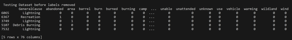
Oregon Weather and Wildfires Specific Cause Comments Years 2000 to 2022
Why Disjoint Training and Testing Data Sets
In machine learning, it is important to have training and testing data disjoint for several reasons, which are related to the goals of building a reliable model. Disjoint training and testing data help ensure that the model can effectively learn patterns from data and make accurate predictions on unseen, real-world examples. Testing on the training data does not prove that the model works on new data, new data is required to prove that, thus a disjoint testing set. Testing data is used to evaluate the performance of the model. It acts as a tool for how well the model will perform on new, unseen data. By keeping the testing data separate from the training data, one can assess how well the model generalizes to unseen instances. If one uses the same data for both training and testing, your model may simply memorize the training data rather than learning general patterns. This can lead to overfitting, where the model performs well on the training data but poorly on new data. Disjoint data prevents data leakage, ensuring that the model does not inadvertently learn from the testing data.
In many real-world applications, machine learning models are used to make important decisions. Disjoint testing data provides a higher level of trust and credibility in the model’s performance, which is essential for applications like medical diagnosis, autonomous driving, and financial predictions. To implement this separation, it is common practice to split the dataset into three parts: training data, validation data (used for model tuning if necessary), and testing data. The exact split ratio may vary depending on the size of your dataset, but the key idea is to ensure that the data used for testing is completely independent of the data used for training. For the supervised learning technique, only a training and testing dataset split will occur. This is partly for simplicity, though for future analyses validation instills a more credible model.
Code
All code associated with the Support Vector Machine (SVM) code and for all other project code can be found in the GitHub repository located here. Also the specific SVM code is in the file named svm.py. Another note, some inspiration for the code is from Dr. Ami Gates Support Vector Machines in Python8 and from the sklearn library documentation9.
Results
US Wildfires By Season for Years 2000 to 2022
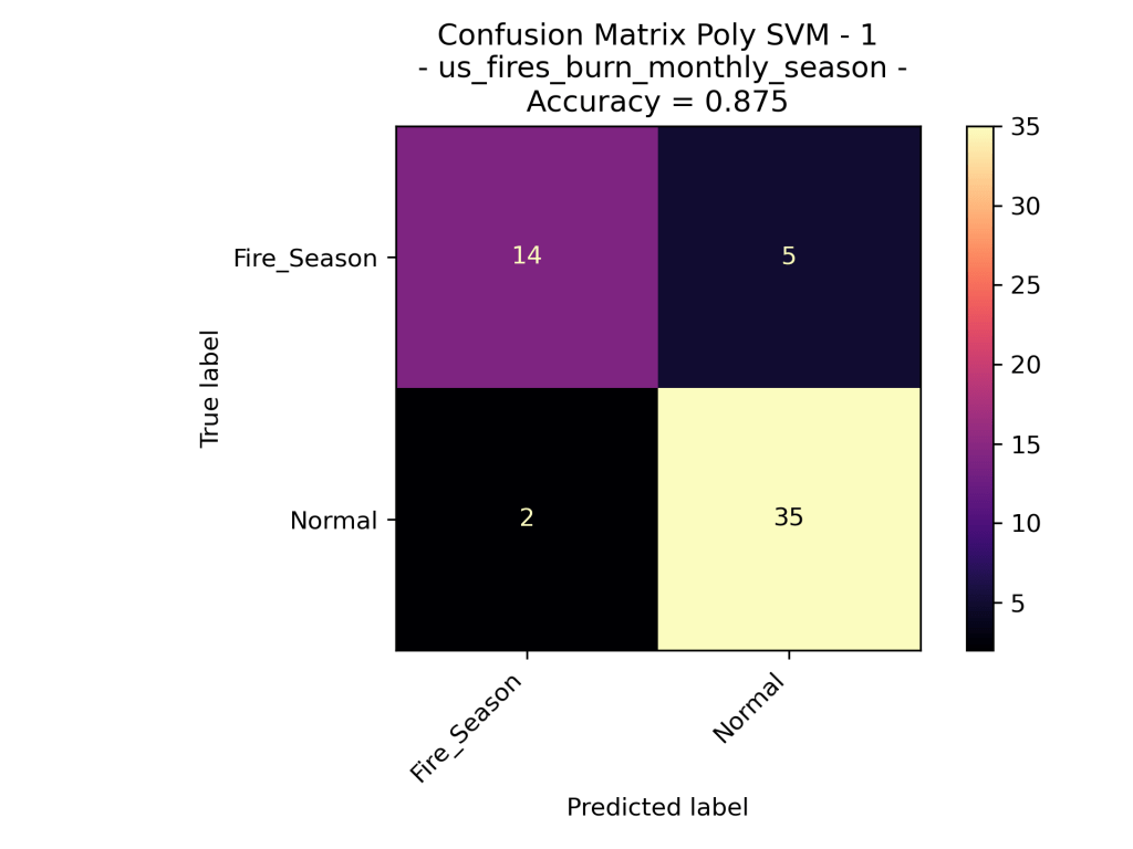

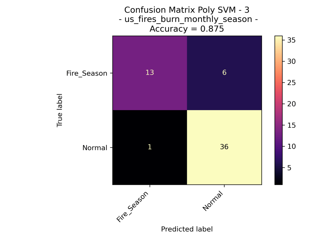
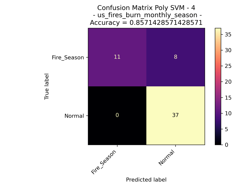
The above confusion matrices go through the results of the different Support Vector Machine Models. The top row demonstrates the results of the Linear SVM (no dot product transformation), then the Radial Basis Function Kernel SVM, then the Polynomial Kernel SVM with degree=1 (in other words – linear). As one can quickly assume the Polynomial Kernel with degree=1 behaved similarly to that of the Linear SVM. Interestingly the RBF Kernel performed significantly worse that the linear and polynomial kernel. The RBF only labeled data as “Normal” which could be very bad analyzing new data assuming that this model is accurate.
Looking at the results of the Polynomial Kernel at different degrees (ranging from 1 to 4 dimensions), we can see that they seem to be very similar in their accuracy of the data. Given that the models are using the exact same training set, we could say that degree=1, 3 perform better than degree=2, 4. However, the difference is minor.
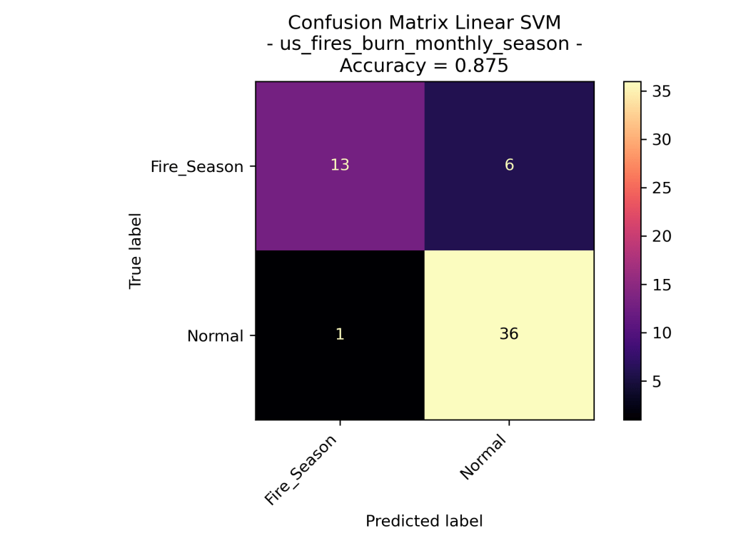
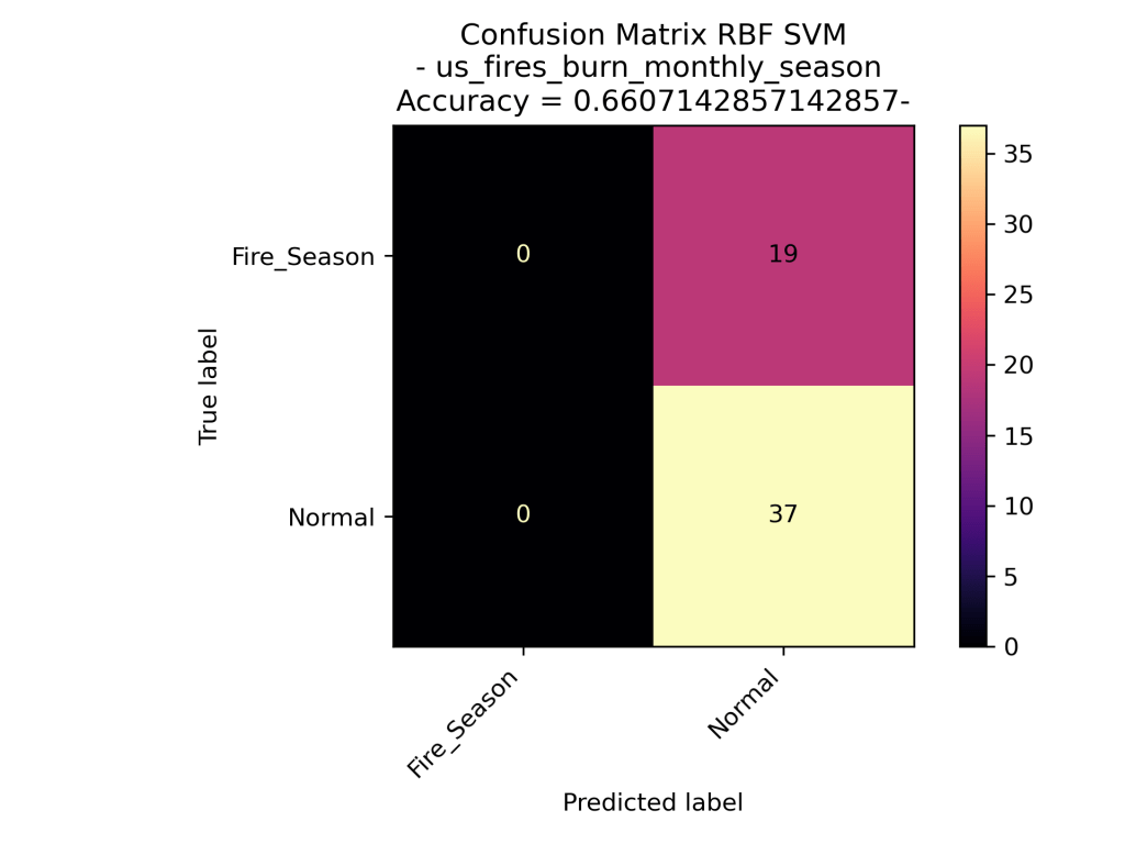
US Wildfires By Month for Years 2000 to 2022
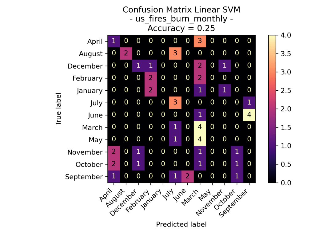
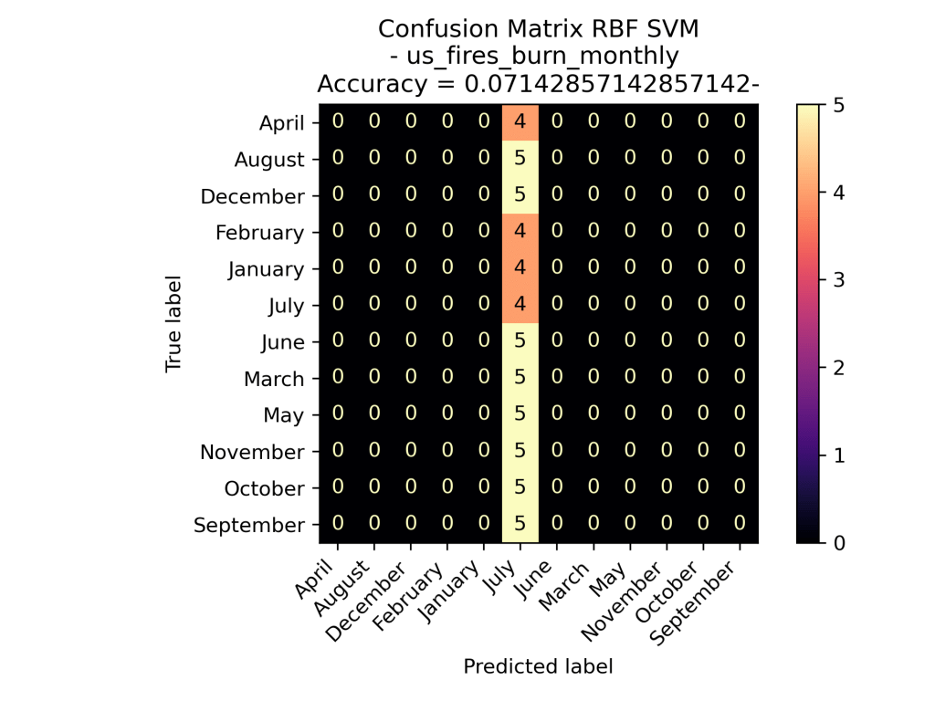

As one can see in the confusion matrix visuals, the Linear SVM performed the best on the data predicting the month based on the acres burned and the number of fires from the years 2000 to 2022. Similar to what’s seen in the Wildfires Seasonal models, the RBF Kernel hyper-focused on one data label for all of its predictions, specifically the month July. A guess as to why the the monthly data is difficult to model is because the number of fires and the acres burned in the United States has been unstable throughout the years. Instead of having each month have a specific number of fires each year, the number of fires have been decreasing and the acres burned have been increasing over time (as seen in the Exploratory Data Analysis).
News Headlines for Wildfires, Burn, Fire, and Weather
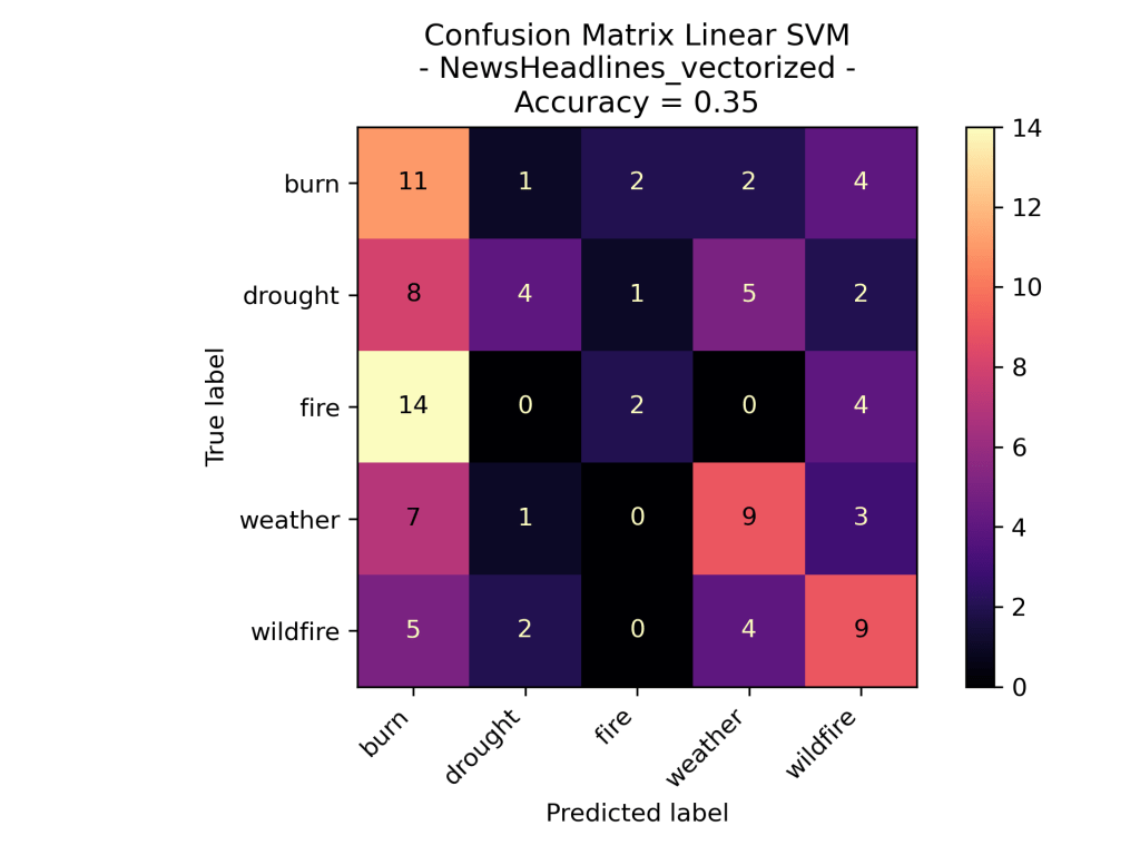
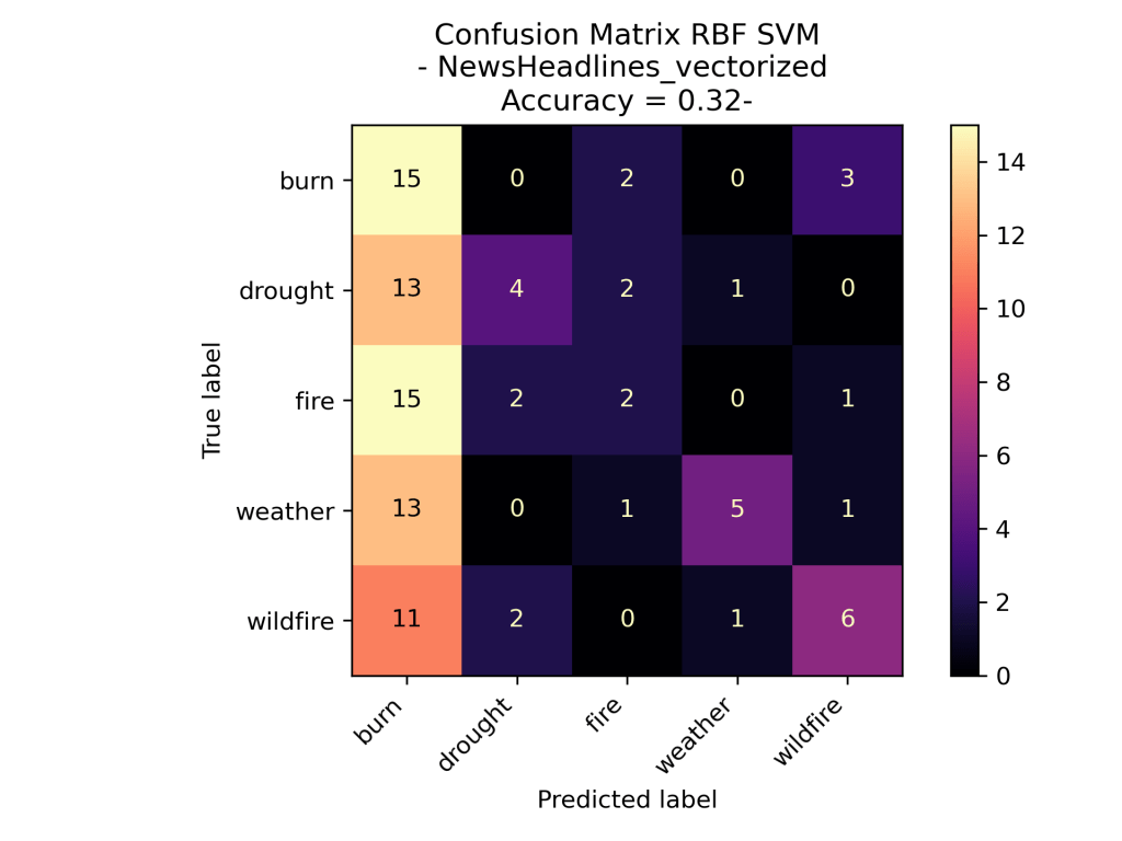
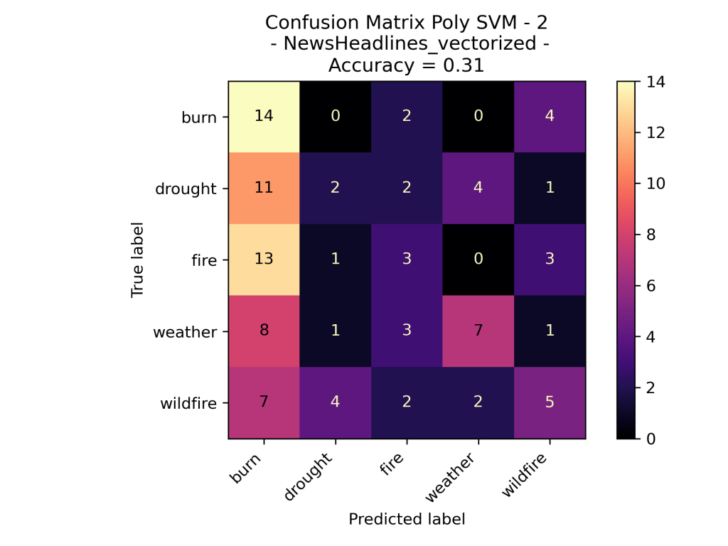
For the Support Vector Machine Model on the News Vectorized Data Wildfires the model was based on the number of times each topic word was used in a Headline on September 16th 2023. The idea of this analysis was to see if certain topics had more distinct words and a new headlines topic could be identified based upon the words in it. As we can see the Linear SVM performed this dataset. However, surprising the RBF did not label all of the test data one class as before. Over all this is still not that accurate of a model as even the best one is performing only slightly better than pure random.
News Headlines for Wildfire and Weather


When grouping topics to known correlative words to break down the Headlines to ones covering “weather” and other covering “wildfires” we can see that the support vector machine has performed better. Here the Radial Basis Function Kernel performed the best out of the three with a decent accuracy of 77.5%.
Oregon Weather and Wildfires Cause Comments


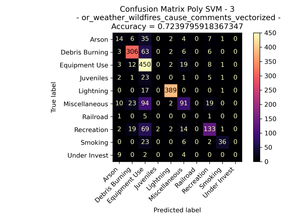
When examining the SVM models applied to fire cause comments in Oregon from 2000 to 2022, we gain insight into its performance in predicting the primary causes based on the language used to describe these incidents. The model for each of the different kernels did well in accurately predicating the overall cause of the fire based on the counts of specific words used in the comments. Out of the three types of kernels performed the linear kernel performed the best, followed by the polynomial kernel, and then by the rbf kernel.
Oregon Weather and Wildfires Specific Cause Comments
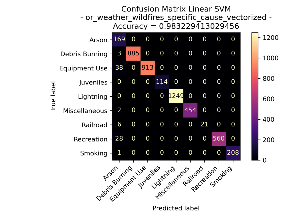

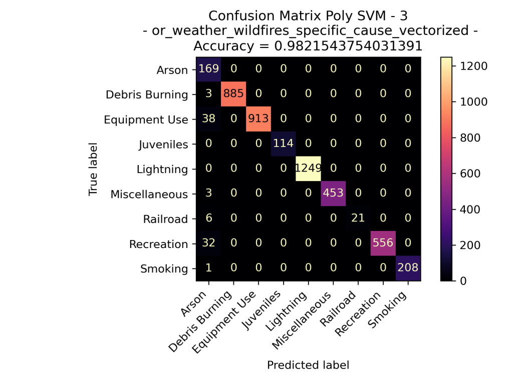
It’s intriguing to observe that for comments related to the specific cause of the fire, the SVM supervised learning models appear to excel in predicting the general cause labels better than just cause comments. Similarly to what we observed in the cause-related comments, “Lightning” stands out as a prominent category among the possible general causes, resulting in a higher number of predictions compared to actual instances. Overall the specific cause comment data for Oregon Wildfires between the years 2000 and 2022 have fantastic results in each of the Support Vector Machine models, each kernel having an above 97% accuracy.
Conclusions
In conclusion, support vector machines (SVMs) have proven to be powerful tools in the realm of machine learning, demonstrating their effectiveness across various applications, including the analysis of wildfire data in the United States. SVMs, encompassing linear, radial basis, and polynomial kernels, offer a robust framework for classification tasks, leveraging the concept of finding optimal hyperplanes to separate data points into distinct classes.
The linear SVM, with its simplicity and efficiency, provides a solid baseline for classification tasks. On the other hand, radial basis and polynomial kernel SVMs introduce a higher level of flexibility, allowing for the modeling of non-linear relationships within the data. These diverse kernel functions enable SVMs to capture intricate patterns and relationships in the wildfire data, making them suitable for the complexity inherent in such environmental datasets.
The application of SVMs to wildfire data has yielded successful results in some datasets and less so in others. As we can see the application of SVMs performed decently when predicting the time of year in seasons for US fires from 2000 to 2022. Also for count data of words in headlines performed decently when attempting to predict “wildfires” versus “weather” as the topic. Both of these results show promise that there are identifiable differences that the models can use to predict future data. Another outstanding model performance was in the case of predicting the general cause of wildfires in Oregon based on the specific cause comments.
SVMs are not only powerful classifiers but also possess advantages such as robustness to overfitting, versatility in handling different types of data, and the ability to generalize well to unseen instances. These qualities make SVMs a valuable tool in addressing the challenges posed by the dynamic and evolving nature of wildfire data.
In essence, the success of SVMs in the analysis of wildfire data underscores their significance as versatile and effective machine learning models. As we continue to refine and expand our understanding of support vector machines, their application in environmental science, particularly in wildfire prediction and management, holds great promise for enhancing our ability to mitigate the impact of these natural disasters.
- Zoltan, Czako. “SVM and Kernel SVM.” Medium, Towards Data Science, 22 Feb. 2022,
https://towardsdatascience.com/svm-and-kernel-svm-fed02bef1200 ↩︎ - 3blue1brown. “Vectors | Chapter 1, Essence of Linear Algebra.” YouTube, YouTube, 6 Aug. 2016,
https://www.youtube.com/watch?v=fNk_zzaMoSs&list=PLZHQObOWTQDPD3MizzM2xVFitgF8hE_ab ↩︎ - VisuallyExplained. “The Kernel Trick in Support Vector Machine (SVM).” YouTube, YouTube, 9 May 2022,
https://www.youtube.com/watch?v=Q7vT0–5VII ↩︎ - StatQuest with Josh Starmer. “Support Vector Machines Part 1 (of 3): Main Ideas!!!” YouTube, YouTube, 30 Sept. 2019, https://www.youtube.com/watch?v=efR1C6CvhmE&t=319s ↩︎
- Sidharth. “The RBF Kernel in SVM: A Complete Guide.” PyCodeMates, PyCodeMates, 12 Dec. 2022,
https://www.pycodemates.com/2022/10/the-rbf-kernel-in-svm-complete-guide.html ↩︎ - VisuallyExplained. “The Kernel Trick in Support Vector Machine (SVM).” YouTube, YouTube, 9 May 2022,
https://www.youtube.com/watch?v=Q7vT0–5VII ↩︎ - StatQuest with Josh Starmer. “Support Vector Machines Part 1 (of 3): Main Ideas!!!” YouTube, YouTube, 30 Sept. 2019, https://www.youtube.com/watch?v=efR1C6CvhmE&t=319s ↩︎
- Gates, Ami. “Support Vector Machines.” Gates Bolton Analytics, gatesboltonanalytics.com/?page_id=304. Accessed 18 Nov. 2023. ↩︎
- “Sklearn.Svm.SVC.” Scikit, scikit-learn.org/stable/modules/generated/sklearn.svm.SVC.html. Accessed 25 Nov. 2023. ↩︎
