Regression

Overview

In the context of machine learning, regression refers to a type of supervised learning algorithm that models the relationship between a dependent variable (target) and one or more independent variables (features or predictors). The goal of regression is to learn a mapping from the input features to the output variable, allowing the algorithm to make predictions on new, unseen data. The main objective in regression is to find a function that approximates the underlying relationship between the input features and the target variable. This function, often referred to as the regression model, is typically represented by a mathematical equation.

The process of training a regression model involves adjusting the coefficients to minimize the difference between the predicted values and the actual values in the training data. Common techniques for this purpose include ordinary least squares (OLS) for linear regression and various optimization algorithms for more complex models. Regression models can be linear or non-linear, depending on the nature of the relationship between the features and the target variable. Regression can also be performed as a Bayesian Model using prior knowledge to increase the accuracy of the model. “Multivariate regression is a technique used to measure the degree to which the various independent variable and various dependent variables are linearly related to each other. The relation is said to be linear due to the correlation between the variables. Once the multivariate regression is applied to the dataset, this method is then used to predict the behavior of the response variable based on its corresponding predictor variables.”¹

Matrix Representation of Linear regression Model

Matrices and vectors will play an important role for us in linear regression. Let’s review some matrix theory as it might relate to linear regression.

Consider the system of linear equations

$Y_i = \beta_0 + \sum^p_{j=1}\beta_j x_{i,j} + \varepsilon_i$

for i = 1,…,n where n is the number of data points (measurements in the sample), and j = 1,…,p where

$p+1$ is the number of parameters in the model.
$Y_i$ is the $i^{th}$ measurement of the response variable.
$x_{i,j}$ is the $i^{th}$ measurement of the $j^{th}$ predictor variable.
$\varepsilon_i$ is the $i^{th}$ error term and is a random variable, often assumed to be $N(0, \sigma^2)$ .
$\beta_j$ , j = 1,…,p are unknown parameters of the model. We hope to estimate these, which would help us characterize the relationship between the predictors and response.

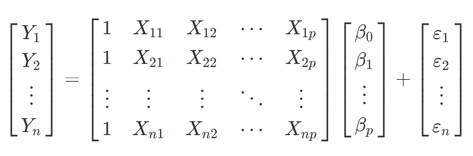
Given the equation above we can rewrite this in a matrix vector form such that

$\mathbf{Y} = \mathbf{X}\boldsymbol\beta + \boldsymbol\varepsilon$

which we can write explicitly as

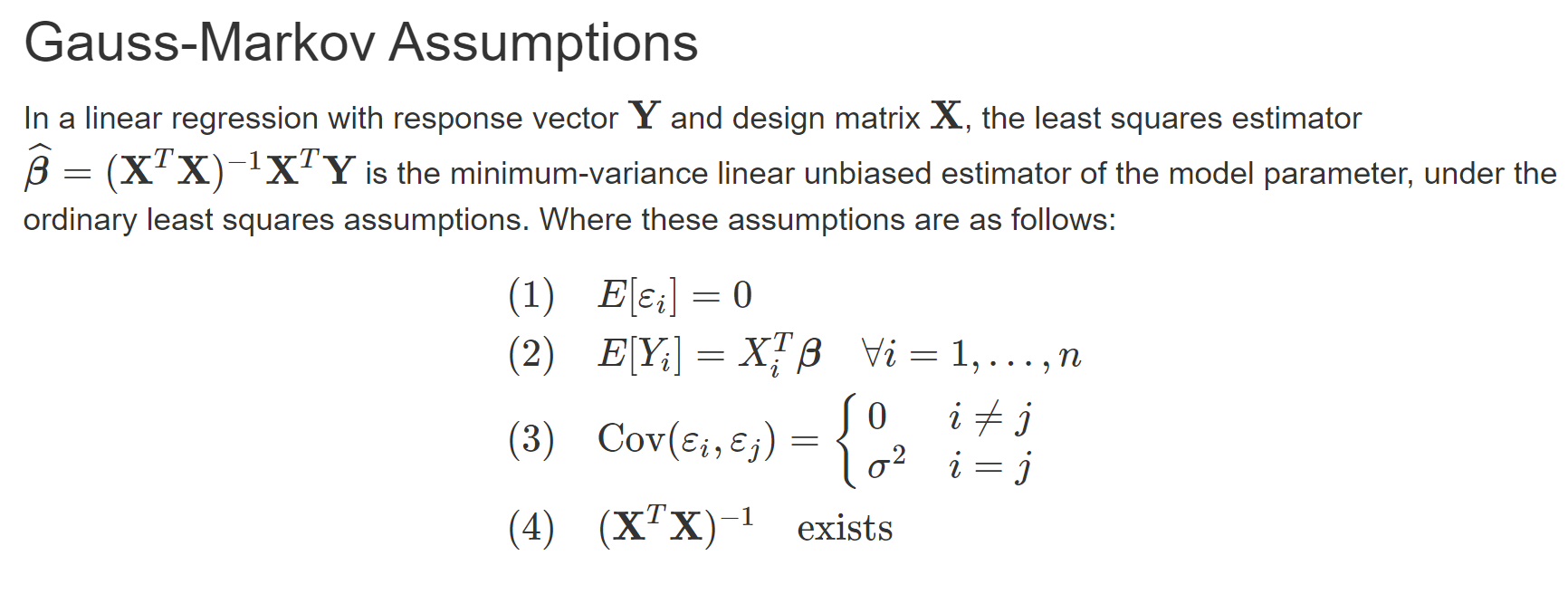
Best Linear unbiased Estimator (B.L.U.E.)

The Gauss-Markov theorem stands as a cornerstone in linear regression, asserting the superiority of the ordinary least squares (OLS) estimator under specific conditions. Essentially, it posits that OLS is the Best Linear Unbiased Estimator (BLUE) for model parameters, providing a minimum-variance and unbiased estimation. In practical terms, the OLS estimator, symbolized as $\widehat{\boldsymbol\beta}$ , is computed as $(\mathbf{X}^T\mathbf{X})^{-1}\mathbf{X}^T\mathbf{Y}$ , where $\mathbf{Y}$ is the response vector and $\mathbf{X}$ is the design matrix. The theorem emphasizes the importance of adhering to ordinary least squares assumptions, including linearity, independence, homoscedasticity, and the absence of perfect multicollinearity. While the Gauss-Markov theorem speaks to optimality within the linear model realm, it acknowledges that alternative nonlinear methods may outperform OLS by different metrics. Nonetheless, for those seeking an unbiased linear model and with OLS assumptions met, the theorem strongly advocates for the use of OLS. It’s important to note that deviations from OLS assumptions, such as the presence of heteroscedasticity, can compromise the optimality of the OLS estimator, prompting consideration of alternative techniques in such scenarios. Mastery of the Gauss-Markov theorem is indispensable for statisticians and econometricians navigating the intricacies of linear regression modeling.²

Sum of Squares

In linear regression analysis, the concept of “sum of squares” plays a crucial role in assessing the goodness of fit of a regression model. The sum of squares is essentially a measure of the total variability in the observed data.

It is divided into two main components: the explained sum of squares (ESS), which accounts for the variability explained by the regression model, and the residual sum of squares (RSS), which represents the unexplained or residual variability. Lastly, there is the total sum of squares (TSS) which is the total variability in the data.

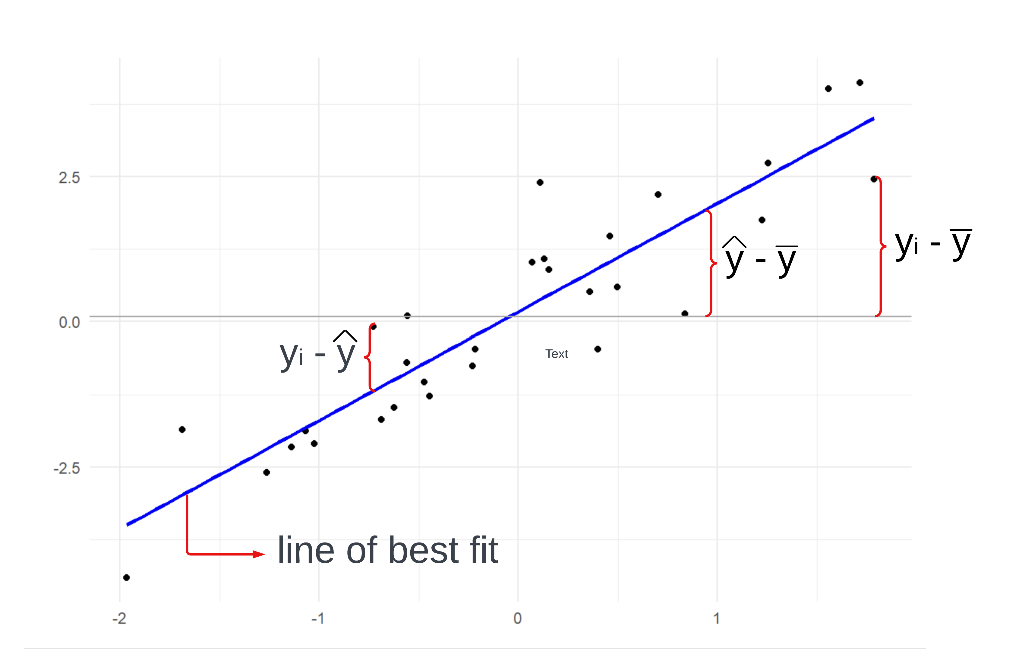
As one can see in the graph their are three major measurements that correspond the the components of ESS, RSS, and TSS which are defined as the following

$TSS = \displaystyle \sum^n_{i=1}(y_i - \bar{y})^2 \quad \quad ESS = \displaystyle \sum^n_{i=1}(\hat{y_i} - \bar{y})^2 \quad \quad RSS = \displaystyle \sum^n_{i=1}(y_i - \hat{y_i})^2$

Coefficient of Determination

The key importance of the sum of squares lies in its utilization to calculate the coefficient of determination, commonly known as the R-squared statistic. R-squared quantifies the proportion of total variability in the dependent variable that is accounted for by the independent variables in the model. A higher R-squared indicates a better fit of the model to the data. Analysts use the sum of squares and related metrics to evaluate the overall performance and significance of the regression model, aiding in the identification of patterns, relationships, and the validity of statistical inferences. In essence, the sum of squares provides a quantitative measure that facilitates the assessment of how well a linear regression model captures the underlying patterns in the observed data, making it a fundamental tool in the interpretation and validation of regression analyses. The $R^2$ coefficient can be defined as the following

$R^2 = 1 - \frac{RSS}{TSS} \quad \text{such that} \quad R^2 \in [0,1]$

Warnings about $R^2$ as a measurement that the model is “good”.

$R^2$ can be close to 1, but the model is the wrong fit for the data.
$R^2$ can be close to 0 even when the model is the correct fit for the data.
$R^2$ should not be used to compare models with a different number of predictors. This is because models with more predictors always have greater $R^2$ values.
$R^2$ says nothing about the causal relationship between the predictors and the response.

For these reasons it is important to look at everything in your disposal when assessing the models performance. To account for the third warning, it is advised to find the value of the adjusted $R^2$ instead.

$R^2_a = 1 - \displaystyle\frac{\displaystyle\frac{RSS}{(n-(p+1))}}{\displaystyle\frac{TSS}{n-1}} = 1 - \displaystyle\frac{n-1}{n-p-1}\Big[1 - R^2 \Big]$

where $p$ is the number of predictors and $n$ is the size of the sample.

The Adjusted R-squared serves as a refined rendition of the traditional R-squared, accounting for the number of predictors incorporated into the model. “The adjusted R-squared increases when the new term improves the model more than would be expected by chance. It decreases when a predictor improves the model by less than expected.”³

Limitations of Regression

Regression analysis, while a powerful statistical tool, has inherent limitations that warrant careful consideration. One notable constraint is the assumption of linearity, implying that the relationship between the independent and dependent variables is accurately modeled by a straight line. Real-world phenomena often exhibit nonlinear patterns, challenging the applicability of regression in capturing complex relationships. Moreover, regression analysis is sensitive to outliers, influential data points that can disproportionately impact model outcomes. Another limitation lies in the assumption of homoscedasticity, implying constant variance in the residuals. Violations of this assumption, often observed in practical data, can lead to inaccurate inferences. Despite these limitations, regression analysis remains indispensable due to its interpretability and simplicity, providing valuable insights into variable relationships. Its utility in hypothesis testing, prediction, and understanding causal connections makes it a versatile analytical tool. In multivariate regression, where multiple independent variables are considered simultaneously, the limitations can be exacerbated. Issues such as multicollinearity, where predictors are highly correlated, can hinder the identification of individual variable contributions. Furthermore, the risk of overfitting increases, as the model may become excessively complex and perform poorly on new data. Despite these challenges, practitioners can mitigate limitations through robust model diagnostics, careful variable selection, and validation techniques, ensuring that the insights gained from regression analysis are reliable and meaningful.

Machine Learning Approach

In machine learning, regression models play a pivotal role in predicting continuous numerical outcomes based on input features. Linear regression is a foundational technique, assuming a linear relationship between the features and the target variable. It’s widely used for its simplicity and interpretability, making it a popular choice in various applications. Moving beyond linear models, multivariate regression extends the framework to accommodate multiple predictor variables, allowing for a more realistic representation of complex relationships. Bayesian regression incorporates Bayesian statistical principles, providing a probabilistic framework to model uncertainty in both the coefficients and predictions. This is particularly useful when dealing with limited data or when a prior belief about the parameters exists. Logistic regression, despite its name, is employed for binary classification problems in machine learning. It models the probability of a binary outcome, making it a key tool for predicting categorical responses. Each regression model brings its own strengths and considerations, allowing practitioners to choose the most suitable approach based on the nature of the data and the specific goals of the machine learning task. The adaptability of regression models, from the simplicity of linear regression to the probabilistic nature of Bayesian regression and the binary prediction capabilities of logistic regression, underscores their versatility in addressing a broad spectrum of predictive modeling challenges.

Data Prep

For this analysis we will be looking into the logistic regression analysis of Fire Season and Human vs Lightning causes of fires.

Logistic regression is a statistical method used for modeling the probability of a binary outcome, which means an outcome with two possible categories, such as success/failure, yes/no, or 0/1. Unlike linear regression, which predicts a continuous outcome, logistic regression models the log-odds of the probability of the event occurring. The logistic function, also known as the sigmoid function, is employed to transform a linear combination of predictor variables into a range bounded between 0 and 1, representing probabilities.

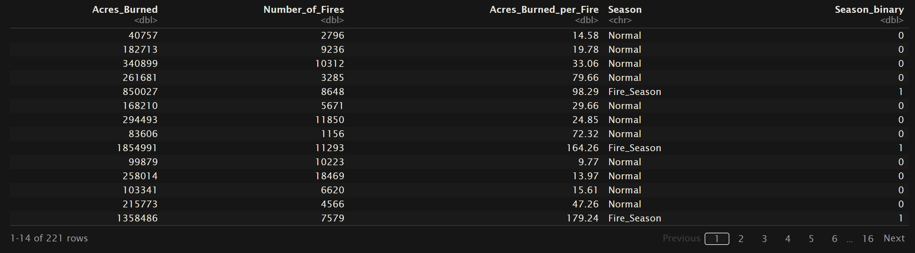
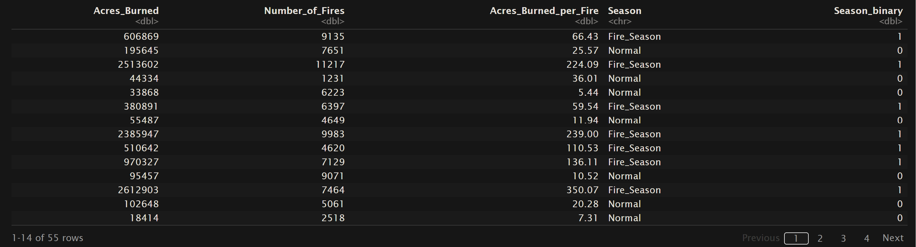
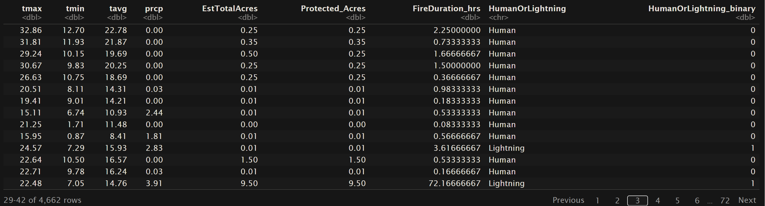
For logistic regression to be applicable, the data need to meet certain assumptions. Firstly, the dependent variable should be binary or dichotomous, meaning it takes on only two possible outcomes. Secondly, there should be a linear relationship between the log-odds of the outcome and the independent variables. This implies that the effect of changing any predictor variable is constant across all levels of that variable. Additionally, the observations should be independent of each other, and there should be little or no multicollinearity among the predictor variables. Logistic regression also assumes that the error terms are independent and follow a logistic distribution. Meeting these assumptions is crucial for obtaining reliable and valid estimates from the logistic regression model. Below is the training and testing dataset for the logistic models. The variables “Season” and “HumanOrLightning” are binary values, but for the ease of calculation a new column is added to represent the string values as 1 or 0. The orginial column has been left for this visual inorder to demonstrate how the values mapped to the binary values. Also all data can be found in the GitHub repository here.

U.S. Wildfires – Normal vs Fire Season Months

Oregon Wildfire and Weather Data (2000 – 2022) – Human or Lightning Causes

Code

All code associated with the decision tree and for all other project code can be found in the GitHub repository located here. Also the specific decision tree code is in the file named regression.Rmd. Another note, some inspiration for the code from Logistic Regression Essentials in R by Alboukadel Kassambara⁴.

Results

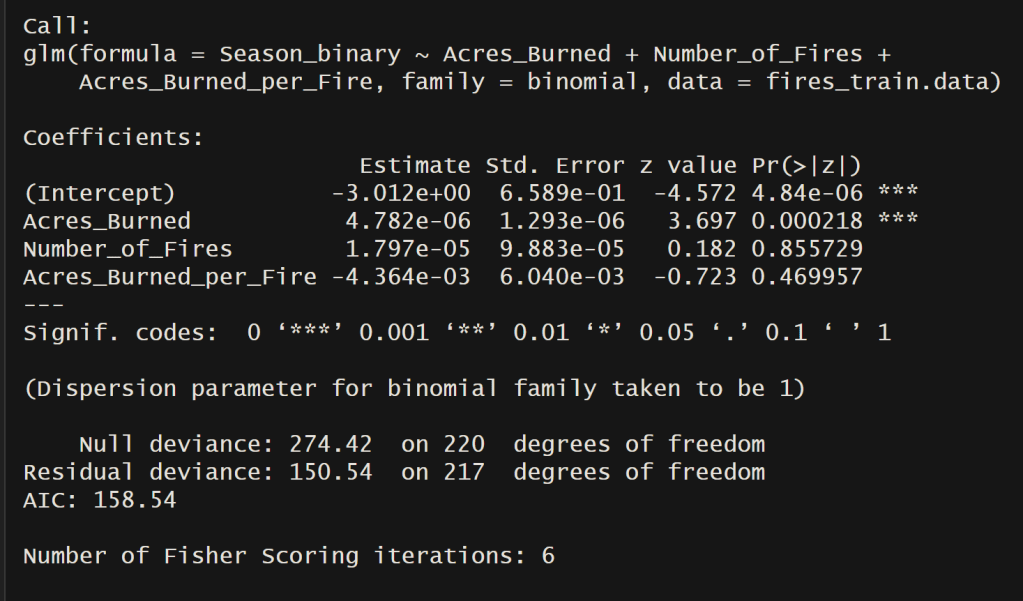
U.S. Wildfires – Normal vs Fire Season Months

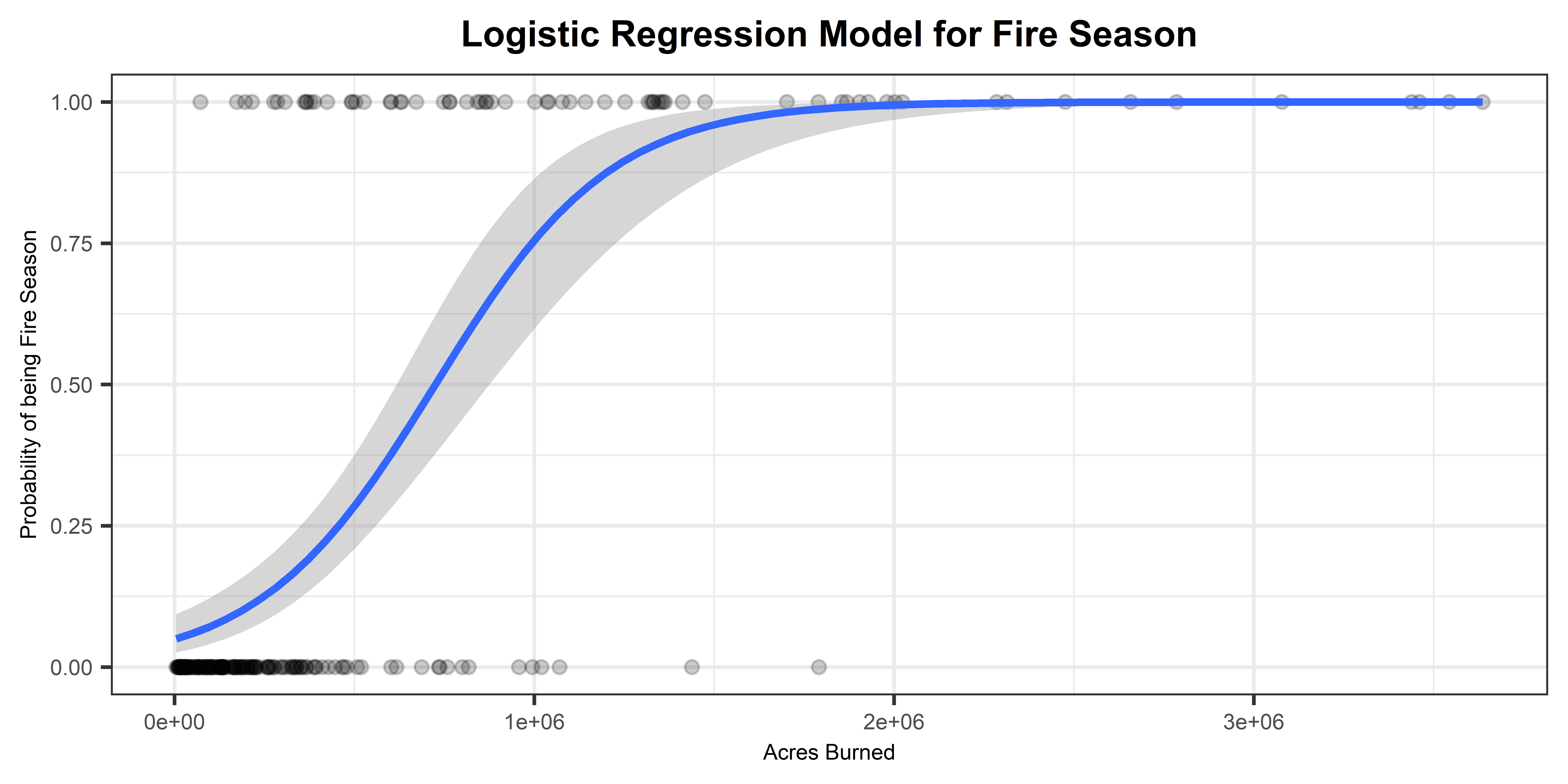
Accuracy = 92.72727%

Examining the model output reveals that “Acres Burned” significantly influenced the binary outcome variable “FireSeason.” Analyzing the logistic curve depicting the probability of a season being categorized as “FireSeason” based on the variable “Acres Burned,” a noticeable shift occurs around 750,000 acres. Beyond this threshold, it becomes more probable that the fire occurred during the “Fire Season” compared to the “Normal” season. The model demonstrated exceptional performance in accurately classifying new test instances, distinguishing between seasons categorized as “Normal” or “Fire Season.”

Oregon Wildfire and Weather Data (2000 – 2022) – Human or Lightning Causes

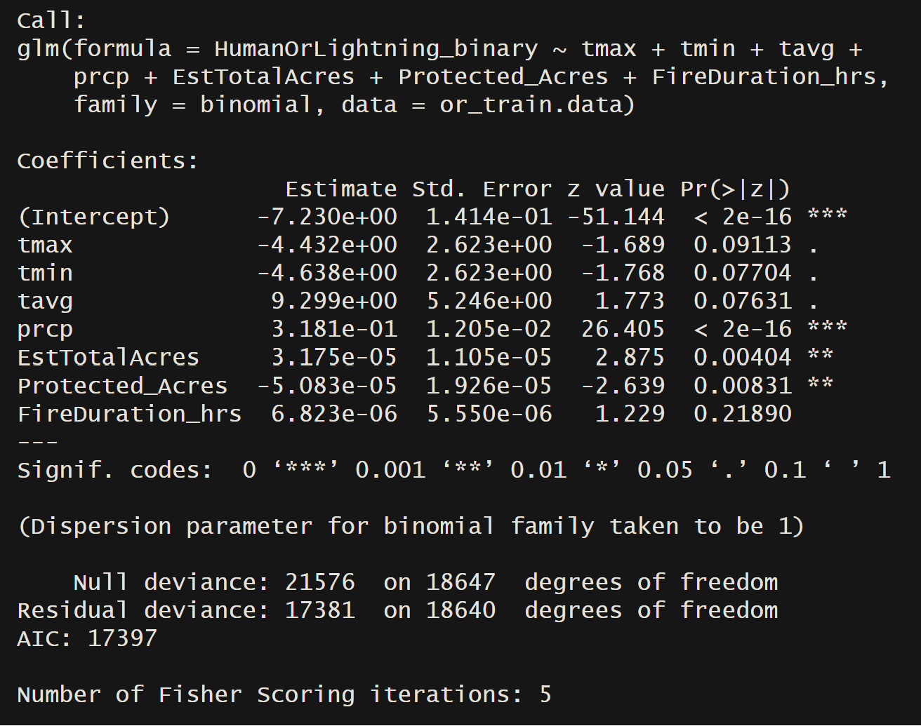
Accuracy = 77.47748%

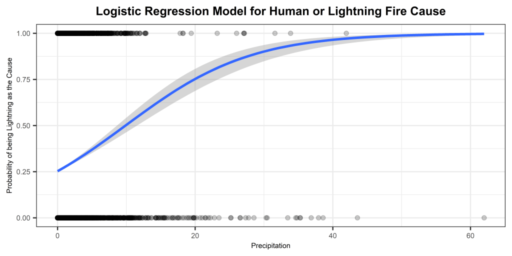
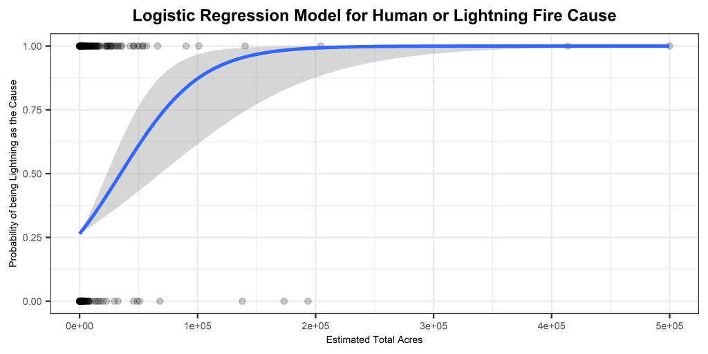
The displayed logistic regression model effectively discerns whether fires in Oregon, spanning from 2000 to 2022, were ignited by human factors or lightning. Notably, the variables “prcp,” “EstTotalAcres,” and “Protected Acres” exhibited significant influence on the response variable. The accompanying logistic probability graphs illustrate distinct patterns. The first graph depicts a gradual rise in the probability of a fire being caused by lightning as precipitation increases. Meanwhile, the second logistic model reveals a swift ascent in the probability of lightning being the cause, nearing 100%, as estimated total acres increase. These findings provide valuable insights into the influential factors determining the cause of fires in Oregon during the specified timeframe.

Conclusions

In conducting two logistic regression analyses on wildfire variables in the United States, our models yielded promising results. The first analysis, with an accuracy of 92.73%, spotlighted the substantial impact of “Acres Burned” on categorizing seasons as “FireSeason” or “Normal.” Notably, the logistic curve illustrated a significant shift around 750,000 acres, indicating a higher likelihood of fires occurring during the “Fire Season.” The model demonstrated exceptional accuracy in classifying new instances, effectively distinguishing between seasons.

In the second analysis focused on Oregon wildfires from 2000 to 2022, the model achieved an accuracy of 77.48%. The key influencers identified were “prcp,” “EstTotalAcres,” and “Protected Acres.” Examining the logistic probability graphs revealed intriguing patterns. The first graph showcased a gradual increase in the likelihood of lightning-caused fires with rising precipitation. Conversely, the second graph depicted a rapid surge in the probability of lightning as the estimated total acres increased, reaching near 100%. These findings offer valuable insights into the factors influencing fire causes in Oregon over the specified timeframe.

These analyses hold significant implications for wildfire management and prediction. The identification of influential variables such as “Acres Burned,” “prcp,” and “EstTotalAcres” provides a foundation for more targeted preventive measures and resource allocation. Stakeholders in wildfire-prone regions, including policymakers and firefighting agencies, can leverage these insights to enhance preparedness and response strategies.

Multivariate regression: Definition, example and steps. Voxco. (2021, December 17). https://www.voxco.com/blog/multivariate-regression-definition-example-and-steps/#:~:text=Multivariate%20regression%20is%20a%20technique,the%20correlation%20between%20the%20variables ↩︎
Gundersen, G. (2022, February 8). The Gauss–Markov Theorem. Gregory Gundersen. https://gregorygundersen.com/blog/2022/02/08/gauss-markov-theorem/#:~:text=Thus%2C%20the%20Gauss%E2%80%93Markov%20theorem,%2Dvariance)%20linear%20unbiased%20estimator. ↩︎
Team, I. (2023, September 28). R-Squared vs. Adjusted R-Squared: What’s the Difference? Investopedia. https://www.investopedia.com/ask/answers/012615/whats-difference-between-rsquared-and-adjusted-rsquared.asp#:~:text=Adjusted%20R%2Dsquared%20is%20a,model%20by%20less%20than%20expected. ↩︎
Kassambara, A. Logistic regression essentials in R – articles – STHDA. (2018, November 3). http://www.sthda.com/english/articles/36-classification-methods-essentials/151-logistic-regression-essentials-in-r/#:~:text=Logistic%20regression%20is%20used%20to,%2C%20diseased%20or%20non%2Ddiseased ↩︎