
Naïve Bayes
Overview
Naïve Bayes (sometimes known as NB) is a popular supervised machine learning algorithm known for its effectiveness in applications like recommendation systems, text classification, and sentiment analysis. Its ability to handle high-dimensional data makes it especially valuable in text classification tasks.1
This generative learning method, finds its foundation in Bayes’ Theorem, which harnesses prior and conditional probabilities to compute posterior probabilities. Essentially, this algorithm probabilistically models the data distribution across various classes or categories. As evident in the formula, Bayes’ Theorem helps us determine the probability of event A given event B, taking into account our prior knowledge of these events.

In essence, Bayes’ Theorem allows for an updated prediction of an event when new information is incorporated. In statistical terms, “prior knowledge” represents the most informed assessment of the probability of an outcome based on existing knowledge before any experimentation takes place, reflecting subjective assumptions regarding the event’s likelihood.
However, what sets Naïve Bayes apart are its “naïve” assumptions, which simplify the classification process. Firstly, it assumes that predictors within the model are conditionally independent, meaning they have no direct relationship with other features in the model. Secondly, it presumes that all features contribute equally to the final outcome.2 Although these assumptions may not hold true in real-world scenarios, such as in natural language processing where words often depend on their context, these simplifications have a purpose. They make the classification problem more computationally manageable by requiring only a single probability calculation for each variable. Surprisingly, Naïve Bayes often performs well, even with these seemingly unrealistic independence assumptions, particularly when dealing with limited sample sizes.
Example
For clear and easy to follow example of by hand analysis of Naïve Bayes watch the video Naive Bayes, Clearly Explained!!! by StatQuest with Josh Starmer. This example goes through an example of identifying emails as “normal” or “spam”. They also use the technique of “add-one smoothing” (which is discussed in “Smoothing in Naïve Bayes”). In summary the video describes how one can use the occurrences of certain words in a label dataset to then assign a probabilistic score to a new email containing these words and therefore identify the label this new email should be assigned.
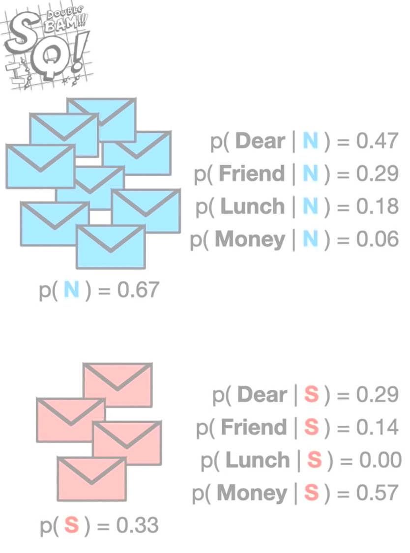
From the video the conditional probabilities of the various words of interest are calculated as well as the probabilities of the labels.
In this example p(N) and p(S) are the priors, and the right hand side conditional probabilities are the likelihoods.
To determine if a new email should be assigned the label “normal” or “spam” the posterior probabilities are calculated for both. For example, given a new email contains the words “Dear” and “Friend”, then we have:
posterior = likeihood*prior / normalizing factor
p(Label|Words) = p(Words|Label)p(Label) / p(Words)
p(N|{“Dear”, “Friend”}) = (.47)(.29)(.67) = 0.09
p(S|{“Dear”, “Friend”}) = (.29)(.14)(.33) = 0.01
Since p(N|{“Dear”, “Friend”}) > p(S|{“Dear”, “Friend”}), then we assign the new email as “normal”. As mentioned above, Naïve Bayes is called “naïve” because of some assumptions. Independence is assumed between the words “Dear” and “Friend”, even though it would be more wise to assume they are not.
** Note that we did not divide by the “normalizing factor”. That is because its the same for both and therefore unnecessary for comparison.
Smoothing in Naive Bayes
Smoothing, often referred to as Laplace or add-one smoothing, is required for Naïve Bayes (NB) models to address a common problem known as “zero probability” or “zero frequency” issue3. This issue arises because, in many real-world text classification and machine learning tasks, there are words or features in the data that may not appear in every class or category (as seen in the example above for spam emails for the word “Lunch”). When you calculate the conditional probabilities for these features based on the observed training data, you may encounter situations where some probabilities become zero.
In the context of Naïve Bayes, each feature (word or term in text classification) is considered independently, and the probability of a particular feature occurring in a given class is calculated by counting the number of times that feature appears in the training examples of that class and dividing it by the total number of training examples in that class. When a feature is absent from a particular class, the probability calculation would result in a zero probability for that feature in that class.
Zero probabilities cause a significant problem when applying the Naïve Bayes algorithm. If any feature in a document is assigned a zero probability in a particular class, it would make the entire probability calculation for that class zero, regardless of the other features. As a result, the classifier would incorrectly classify documents as having zero probability for a class they may actually belong to.
To prevent our posterior probabilities from ever reaching zero, we employ a method of adding 1 to the numerator and k to the denominator. This means that even when dealing with scenarios where a specific ingredient is absent from our training set, the posterior probability is calculated as 1 / (N + k), ensuring it never becomes zero. This approach safeguards our ability to make predictions, as it avoids the problematic outcome of zero probability when included in the calculation.4 With smoothing our formula becomes
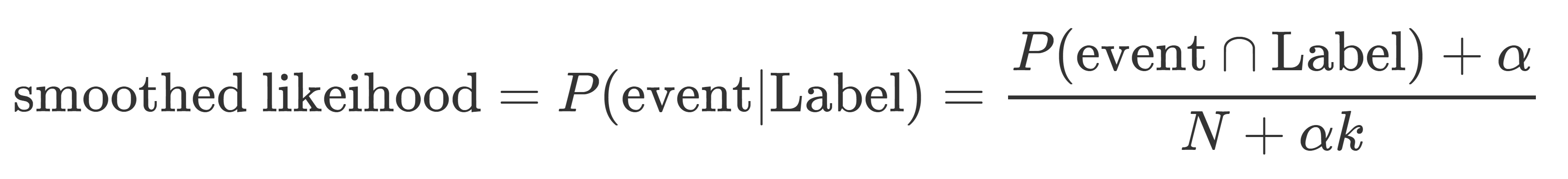
Where
- alpha : represents the smoothing parameter (for the “add-one smoothing” case, alpha = 1)
- k : represents the number of features in the dataset
- N : represents the size of the sample that satisfies the condition.
Standard Multinomial Naïve Bayes
In many mathematical based algorithms non numerical data poses different approaches and challenges for training and modeling. The Multinomial Naïve Bayes model offers a unique approach to classifying non-numerical data with the notable benefit of reduced complexity. It excels in handling small training sets and obviates the need for frequent retraining.
One example of the uses case of Multinomial Naïve Bayes is in text classification using a statistic probabilistic approach. Text classification aims to assign document fragments to relevant classes by evaluating the likelihood that a document pertains to a class shared by other documents of the same subject matter. Within this framework, documents are composed of multiple words or terms, which collectively contribute to understanding their content. Each class corresponds to one or multiple documents, all related to the same subject. The classification process involves associating documents with existing classes through statistical analysis, testing the hypothesis that a document’s terms have occurred in other documents from a particular class. This approach increases the probability of correctly assigning a document to the same class as others that have already been classified.
For our analysis of data on wildfires, this approach will be used to create a model that can assign a label to text information. For example, given a report of a fire the model would be able to predict the cause of the fire based on the brief description.
Bernoulli Naïve Bayes
For Bernoulli Naïve Bayes it is important to first discuss Bernoulli Probability.
At its core, Bernoulli probability deals with the analysis of random experiments or trials that result in one of two possible outcomes, typically labeled as “success” and “failure.” These experiments are characterized by being binary, meaning there are only two mutually exclusive and exhaustive outcomes.
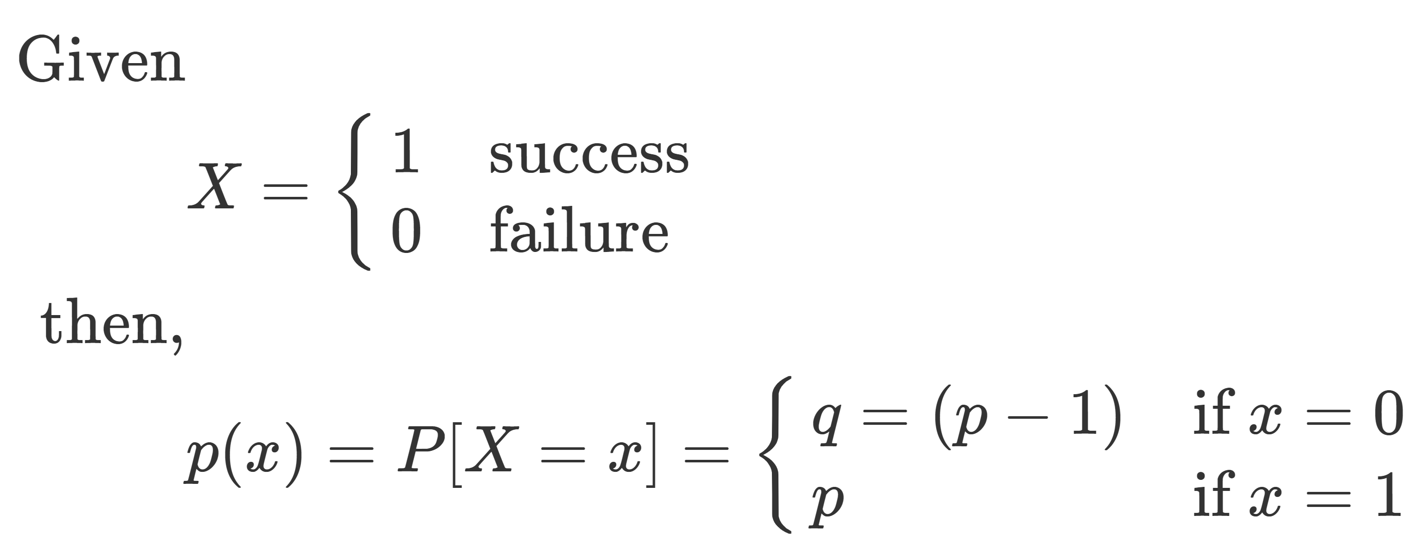
Bernoulli probability is widely used to model various real-world situations, such as coin flips (heads or tails), product quality inspections (defective or non-defective), or the diagnosis of a medical ailment. It forms the basis for more advanced probability distributions, including the Binomial distribution, which describes the number of successes in a fixed number of Bernoulli trials, making Bernoulli probability a fundamental concept with broad applications in statistics and decision-making.
In the world of Naïve Bayes, Bernoulli Naïve Bayes functions similarly as it is based on the Bernoulli Distribution and accepts only binary values [0, 1]5. In this approach, the focus is on binary data, where each feature (or term) is considered as either present (success) or absent (failure). It is commonly used for text classification tasks, where the presence or absence of specific words or features in a document determines its categorization into one of two classes, such as spam or non-spam, positive or negative sentiment, or relevant and irrelevant. Bernoulli Naïve Bayes leverages conditional probabilities to estimate the likelihood of a document belonging to a particular class based on the presence or absence of specific features. Despite its simplification of the data, it often proves effective in many text-based applications, especially when dealing with binary feature data and achieving good results with relatively small training sets.
Data Prep
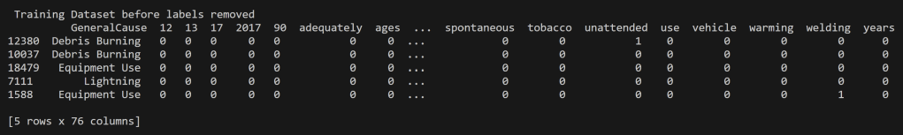
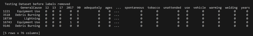
For the analysis of Wildfires in the United States from 2000 to 2022, the naïve bayes modeling was performed on multiple datasets each with different purposes of them. These include quantitative values for the Acres Burned identifying the time of year the fire took place, to that of predicting the topic of an article based on the words used its headline. In order to perform supervised learning appropriately each of the datasets were split into disjoint training and testing datasets with their labels removed (but kept for reference and accuracy analysis). In supervised learning, labels are essential for two primary reasons. They provide the correct output for a given input, allowing the algorithm to learn and make predictions. Labels also enable model evaluation and performance assessment, serving as the basis for key metrics.
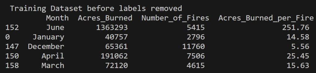
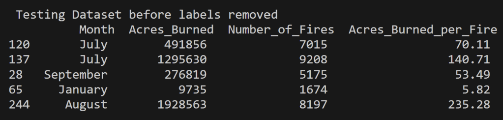
Below is the training and testing datasets that used a random split to have 80% of the data for training and 20% for testing. The goal for a good training set is for all of the possible data values to be represented and be represented in a proportion such that overfitting/underfitting for particular values doesn’t occur. All cleaned data used in this analysis can be found in the project GitHub repository here. Note that the datasets below have the labels still attached for reference, but they were removed from the testing set when running the predictions using the naïve bayes model.
US Wildfires By Season for Years 2000 to 2022
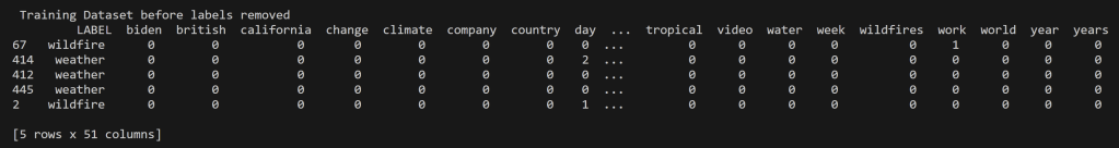
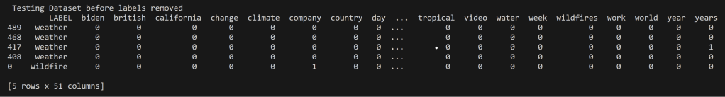
News Headlines from September 16th, 2023
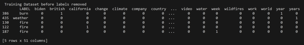
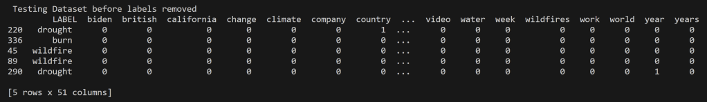
News Headlines for topics “wildfire” and “weather” from September 16th, 2023
Oregon Weather and Wildfires Cause Comments Years 2000 to 2022
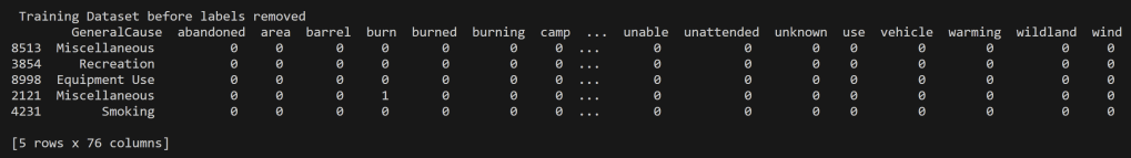
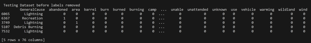
Oregon Weather and Wildfires Specific Cause Comments Years 2000 to 2022
Why Disjoint Training and Testing Data Sets
In machine learning, it is important to have training and testing data disjoint for several reasons, which are related to the goals of building a reliable model. Disjoint training and testing data help ensure that the model can effectively learn patterns from data and make accurate predictions on unseen, real-world examples. Testing on the training data does not prove that the model works on new data, new data is required to prove that, thus a disjoint testing set. Testing data is used to evaluate the performance of the model. It acts as a tool for how well the model will perform on new, unseen data. By keeping the testing data separate from the training data, one can assess how well the model generalizes to unseen instances. If one uses the same data for both training and testing, your model may simply memorize the training data rather than learning general patterns. This can lead to overfitting, where the model performs well on the training data but poorly on new data. Disjoint data prevents data leakage, ensuring that the model does not inadvertently learn from the testing data.
In many real-world applications, machine learning models are used to make important decisions. Disjoint testing data provides a higher level of trust and credibility in the model’s performance, which is essential for applications like medical diagnosis, autonomous driving, and financial predictions. To implement this separation, it is common practice to split the dataset into three parts: training data, validation data (used for model tuning if necessary), and testing data. The exact split ratio may vary depending on the size of your dataset, but the key idea is to ensure that the data used for testing is completely independent of the data used for training. For the supervised learning technique, only a training and testing dataset split will occur. This is partly for simplicity, though for future analyses validation instills a more credible model.
Code
All code associated with the Multinomial Naïve Bayes and for all other project code can be found in the GitHub repository located here. Also the specific naïve bayes code is in the file named naive_bayes.py. Another note, some inspiration for the code is from Dr. Ami Gates Naive Bayes in Python6 and from the sklearn library documentation.
Results
Now, having established the framework and prepared the data, it’s time to delve into the results of the Naive Bayes supervised learning models applied to wildfire data spanning the United States from 2000 to 2022. These models are poised to shed light on patterns and insights in this critical dataset, offering valuable information for understanding and addressing wildfire occurrences in the region.
US Wildfires By Month for Years 2000 to 2022
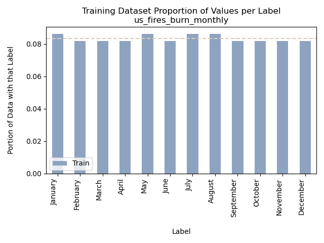

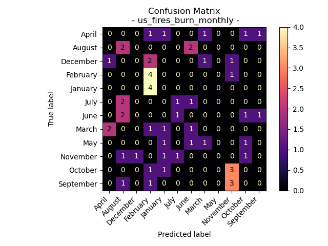
Accuracy = 12.5%
Unfortunately using the label of “Month” for the data of burned area and number of fires in the United States from 2000 to 2022 resulted in a pretty poor Naive Bayes model result. This accuracy level is only slightly better than rolling a 12 sided dice to select the month label. The training and testing data both demonstrated uniform distributions but that wasn’t true for the predicted results, therefore we can assume that the poor performance of the model wasn’t due to a unbalanced training set.
One hypothesis that is worth looking into is that from the Exploratory Data Analysis winter months had lower values of acres burned and for number of fires. It is possible that these months have too many shared ranges for possible values and therefore are getting mislabeled. To investigate this, we relabeled the months June – September as “Fire Season” and all other months as “Normal” to see if this would results in a more accurate model.
US Wildfires By Season for Years 2000 to 2022
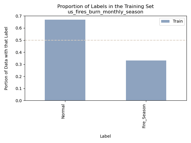
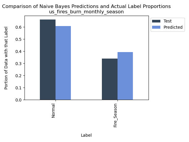
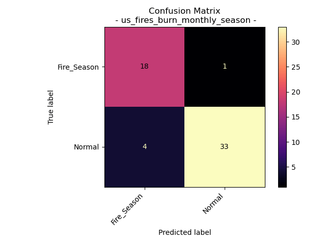
Accuracy = 91.07142857142857%
As anticipated during the reduction of labels to a binary classification, based on the previously conducted Exploratory Data Analysis, we were able to create a notably more precise model for predicting the time of year using the variables “Acres Burned,” “Acres Burned per Fire,” and “Number of Fires.” It’s worth noting that our training data was imbalanced, yet it still yielded impressive accuracy. Intriguingly, the model occasionally misclassified data as “Fire Season” when the true label was “Normal,” despite the overall distribution favoring “Normal.” One hypothesis to explain this anomaly is that the misclassified data point may have originated from an anomalously high-fire activity month within the “Normal” category.
Analyzing the outcomes of the Naive Bayes Model applied to US wildfires between 2000 and 2022, specifically in the context of labeling both “Months” and “Fire Season,” it becomes evident that we can construct a predictive model for determining the time of year using the variables “Acres Burned,” “Acres Burned per Fire,” and “Number of Fires.” However, it is apparent that our results can be substantially improved by simplifying the prediction to the broader category of “time of year” rather than individual months.
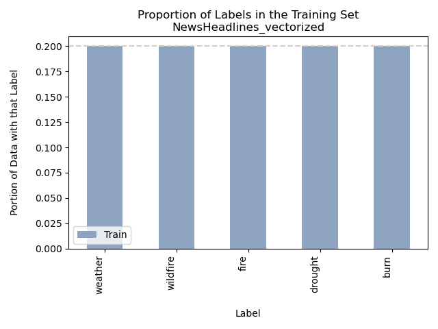
News Headlines for Wildfires, Burn, Fire, and Weather


Accuracy = 31%
In this instance, we’re presented with a well-balanced dataset encompassing the chosen topics found in news headlines, including “weather,” “wildfires,” “fire,” “drought,” and “burn.” Upon an initial glance at the proportion of value bar graphs, it might appear that the Naive Bayes Supervised model effectively labeled the data (with the exception of “burn”). However, upon closer examination of the Confusion Matrix and the accuracy score, it becomes evident that the model’s performance was only marginally better than random chance, akin to the outcome of rolling a five-sided dice to predict the news headline labels. Ideally, the diagonal squares in the Confusion Matrix should exhibit the highest values, but, regrettably, this was not the case.
The topic “fire” was frequently misclassified as “burn” in the headlines. This issue likely stems from the inherent similarity between headlines that pertain to these topics. It’s reasonable to assume that an article discussing a fire would also touch upon subjects that have been burned. In an effort to address the challenge of dealing with words that have closely related contexts, a decision was made to streamline the topics to “wildfires” and “weather.” This decision aimed to simplify the model and minimize errors in the confusion matrix. The rationale behind this choice stemmed from prior analysis of the data, which revealed that the weather data predominantly centered around the discussion of the Hilary Hurricane in California, while the wildfire data focused on the Maui Fire.
News Headlines for Wildfire and Weather


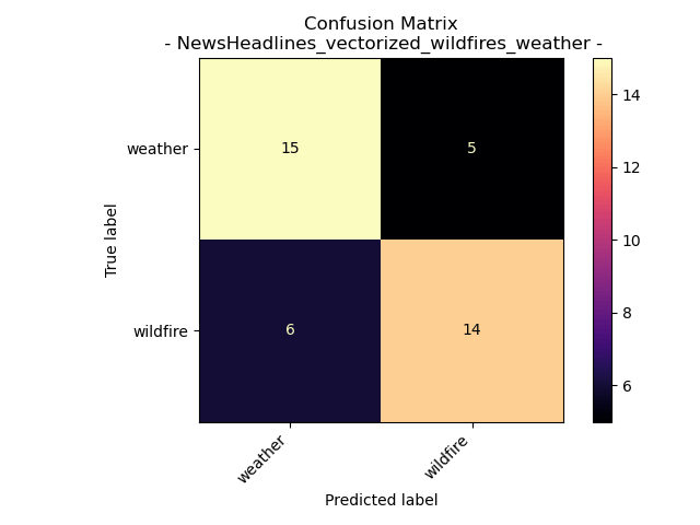
Accuracy = 72.5%
Upon transitioning to a binary classification system, it becomes evident that the Naive Bayes model exhibits notably improved performance, as reflected in the confusion matrix and accuracy. This transformation to a two-class problem yielded a substantial 134% increase in accuracy. Notably, the labels “weather” and “wildfire” were predicted with a higher rate of accuracy than misclassification.
Since headlines are always changing, this model is still plagued by a situation of overfitting for the day the headlines were pulled. The model might be mostly accurately predicting the labels of headlines from September 16th 2023, however, this does not demonstrate that it will accurately predict headline topics for say October 22nd 2023, or even September 16th 2000.
Oregon Weather and Wildfires Cause Comments
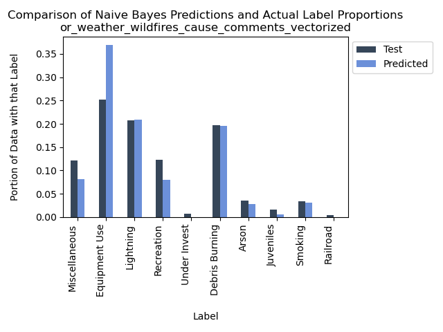
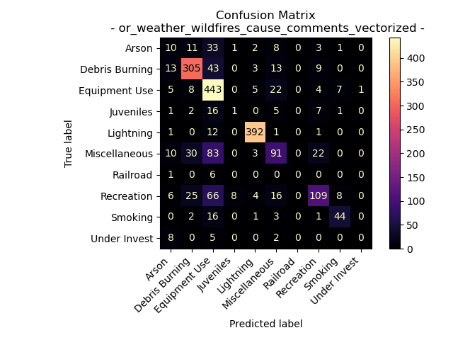
Accuracy = 71.17346938775511%
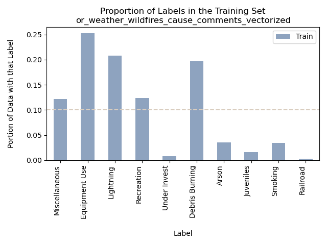
When examining the Naive Bayes model applied to fire cause comments in Oregon from 2000 to 2022, we gain insight into its performance in predicting the primary cause based on the language used to describe these incidents. The model demonstrated a commendable ability to accurately classify the general cause labels, as evident from the accuracy levels and the confusion matrix.
However, an interesting observation emerges from the proportion bar graphs above, indicating that the “Equipment Use” label is notably predominant. This high saturation of the label raises questions about its potential influence on some of the Naive Bayes predicted classifications.
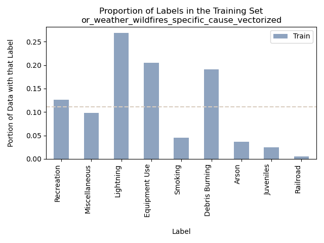
Oregon Weather and Wildfires Specific Cause Comments
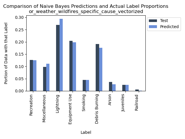
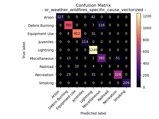
Accuracy = 92.45323586325521%
It’s intriguing to observe that for comments related to the specific cause of the fire, the Naive Bayes supervised learning model appears to excel in predicting the general cause labels. Notably, there is a subtle difference in the distribution of general cause labels when comparing specific comments to those focusing on the cause itself. The precise explanation for this variation remains uncertain, but it may be attributed to the human element in crafting these comments, which can introduce inherent inconsistencies. Similarly to what we observed in the cause-related comments, “Lightning” stands out as a prominent category among the possible general causes, resulting in a higher number of predictions compared to actual instances.
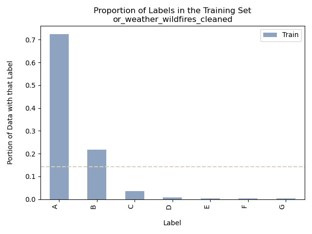
Oregon Weather and Wildfires – Weather Values and Fire Size
For this model we are using the data values of Temperature (maximum, minimum, and average) as well as precipitation to predict the size of the fire is the labels of A-G (smallest to largest) in Oregon from 2000 to 2022.
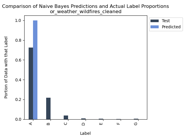
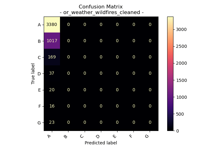
Accuracy = 72.5010725010725%
This serves as a clear illustration of how an imbalanced dataset can have a substantial impact on the accuracy of a supervised learning model. Given the dataset’s pronounced overrepresentation of class “A” fire sizes, the model is biased towards assigning more instances to “A” than is warranted. This bias is evident in both the bar graph and the confusion matrix, showcasing the model’s tendency to over-assign “A” labels and its failure to correctly label instances of other fire size categories.
In this case, the model’s accuracy is primarily attributed to its proficiency in identifying a single category, and that category happens to dominate the dataset. An examination of the proportion bar graphs reveals that “A”-sized fires constitute roughly 70% of the dataset, and the model’s accuracy aligns closely with this figure, indicating its precision in labeling this particular category. The confusion matrix provides further insight, showing that “A” was the only predicted label that missed over 25% of the other categories present in the testing dataset, highlighting a notable imbalance in the model’s performance.
Oregon Weather and Wildfires – Weather Values and Fire Size – Balanced

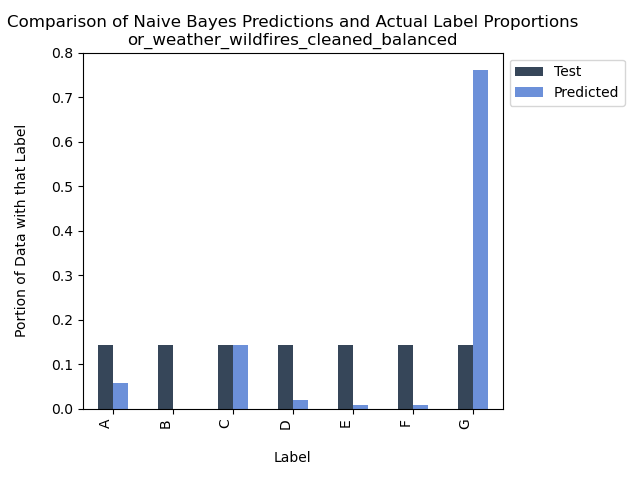
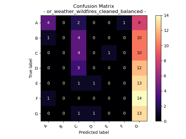
Accuracy = 20%
In our effort to address the modeling challenge posed by the imbalanced dataset, we initially sought to achieve balance in label representation for both the training and testing datasets. However, we now confront a different predicament – an evident bias towards over-labeling for class G. The cause could be related to our sampling method or possibly another factor. While there remains potential for improving the supervised modeling on this dataset in the future, for the time being, we opt to discontinue our endeavor to utilize Oregon weather measurements for predicting fire sizes in Naive Bayes Modeling.
Conclusions
In conclusion, our exploration of Naive Bayes supervised learning models across diverse datasets has unveiled both notable successes and intriguing challenges within various domains. Our journey began with an attempt to predict wildfire occurrences based on monthly labels, yielding a rather modest accuracy of 12.5%, illustrating the complexity of capturing the intricacies of such a dynamic natural phenomenon. However, our transition to a binary classification system as “Fire Season” and “Normal” remarkably improved the model’s accuracy to 91.07%, offering more precise predictions and the reasoning to continue to look into the concept of a “Fire Season” in the United States. Particularly how can this knowledge help to protect people and the environment.
Shifting our focus to the categorization of news headlines, our initial accuracy of 31% hinted at room for growth. Yet, the decision to simplify the model by classifying topics as “wildfires” and “weather” led to a substantial accuracy boost of 72.5%, indicating the model’s ability to excel under focused conditions. Thought simiplfying the model yielded significantly better results, the bias that these new headlines were selected from a single day needs to be made clear in the use of this model.
When we delved into the realm of wildfire causes in Oregon for the years 2000 to 2022, we uncovered a 71.17% accuracy in predicting general cause labels, while the prominence of the “Equipment Use” label raised intriguing questions about its influence. Further investigation into specific cause comments yielded an impressive accuracy of 92.45%, though a subtle shift in label distribution raised doubts about data consistency.
Our analysis of weather and fire size labeling showcased the potential pitfalls of imbalanced datasets, where the dominance of class “A” fire sizes led to inaccuracies in labeling other categories. Finally, in our pursuit of balance within the weather and fire size labels, we encountered an unexpected bias towards over-labeling for class G, emphasizing the intricate nature of tackling imbalances.
In summary, these endeavors demonstrate the multifaceted nature of predictive modeling and the crucial role of data preparation, feature selection, and model evaluation. While our Naive Bayes models exhibited varying levels of performance, each dataset’s unique characteristics demanded adaptability and ingenuity. The successes and challenges encountered throughout this analysis serve as a reminder of the dynamic landscape of machine learning, where ongoing refinement and a deep understanding of domain intricacies are paramount.
- Kavlakoglu, E. (2023, September 27). https://developer.ibm.com/tutorials/awb-classifying-data-multinomial-naive-bayes-algorithm/. IBM developer. https://developer.ibm.com/tutorials/awb-classifying-data-multinomial-naive-bayes-algorithm/ ↩︎
- Singh Chauhan, N. (2022, April 8). Naïve Bayes Algorithm: Everything you need to know. KDnuggets. https://www.kdnuggets.com/2020/06/naive-bayes-algorithm-everything.html ↩︎
- Goyal, C. (2021, April 16). Improve naive Bayes text classifier using laplace smoothing. Analytics Vidhya. https://www.analyticsvidhya.com/blog/2021/04/improve-naive-bayes-text-classifier-using-laplace-smoothing/
↩︎ - Goyal, C. (2021, April 16). Improve naive Bayes text classifier using laplace smoothing. Analytics Vidhya. https://www.analyticsvidhya.com/blog/2021/04/improve-naive-bayes-text-classifier-using-laplace-smoothing/ ↩︎
- Singh Gill, S. (2023, June 30). Bernoulli Naive Bayes. Coding ninjas studio. https://www.codingninjas.com/studio/library/bernoulli-naive-bayes ↩︎
- Gates, Ami. “Decision Trees in Python – Gates Bolton Analytics.” Gates Bolton Analytics, gatesboltonanalytics.com/?page_id=282. Accessed 20 Oct. 2023. ↩︎
