

Decision Trees
Overview
A decision tree is a non-parametric supervised learning algorithm, which is utilized for both classification and regression tasks. It has a hierarchical, tree structure, which consists of a root node, branches, internal nodes and leaf nodes.1 To identify the most effective features and thresholds for data partitioning, decision trees leverage a range of splitting criteria. These criteria encompass well-known metrics like entropy, information gain, and Gini impurity, each playing a pivotal role in pinpointing the ideal features and thresholds that lead to the greatest reduction in impurity and uncertainty. Now, when it comes to the world of decision trees, there are several notable algorithms, including ID3, C4.5, and CART. These algorithms utilize different splitting criteria and techniques to create decision trees.2

In a decision tree, the process kicks off at the root node, which serves as the starting point with no incoming branches. Moving forward, the outgoing branches from this root node extend into what we call internal nodes, often referred to as decision nodes. These nodes (both the root and the internals) assess the available features, ultimately shaping the subsets. These subsets are symbolized by leaf nodes, also known as terminal nodes, and collectively, they encapsulate the entire set of potential outcomes present within the dataset. Which in decision trees these leaves are assigned class labels.
Decision trees possess a remarkable quality in their ability to be easily understood by a diverse audience. They can convey valuable insights that resonate with a broad spectrum of individuals.
“Decision tree learning employs a divide and conquer strategy by conducting a greedy search to identify the optimal split points within a tree. This process of splitting is then repeated in a top-down, recursive manner until all, or the majority of records have been classified under specific class labels”3. Smaller trees are easier for classification of “pure leaf nodes” (a single class of data points), and it becomes increasingly more difficult to “maintain purity” as the size and complexity of the tree increases. Note that no data entries are created nor destroyed as the tree is built.

When this situation occurs, it is referred to as “data fragmentation”, a condition that can frequently result in overfitting. Therefore when developing decision tree models it is best to avoid adding unnecessary complexity. Put simply, decision trees only introduce complexity when it serves a clear purpose, recognizing that the simplest explanation often proves the most effective. To mitigate complexity and forestall overfitting, a common practice is pruning. Pruning is the deliberate removal of branches that split on features with relatively low importance, a strategic move in enhancing model performance and maintaining its generalizability. To maintain accuracy one can form an ensemble through a random forest algorithm; this classifier predicts more accurate results, particularly when the individual trees are uncorrelated with each other.
Measure the “Goodness” of a Split
Given a dataset with multiples variables or attributes it is important to determine the most effective splits in order to efficiently reach “pure leaves” (or close to pure). That is why measures for the “goodness” of a spilt are used to identify how effective that split is for the decision tree. Three different measures that will be discussed here are Entropy, Information Gain, and Gini.
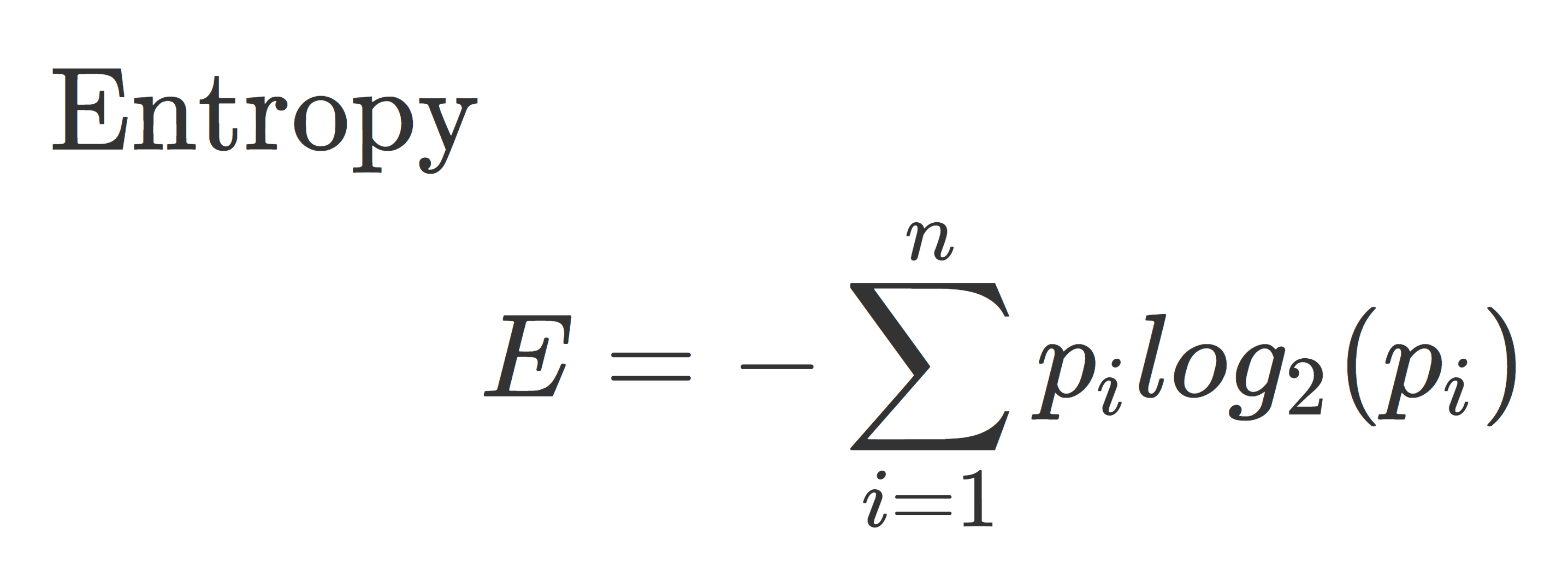
Entropy
Entropy measures the randomness of the data. “The higher the entropy, the harder it is to draw any conclusions from that information.”4 A “leaf” with higher entropy will have a lower purity, it will still have a mix of values. Pure leaf nodes have entropy of 0, and the entropy for a node where the classes are divided equally would be 1.5 Where p is the probability of randomly selecting data in class i.
Information Gain
In essence, when constructing a Decision Tree’s root node, the process involves evaluating the entropy of each variable and its potential divisions. To do this, assess the potential divisions within each variable, calculate the average entropy for the resulting nodes, and then measure the change in entropy compared to the parent node. This change in entropy is referred to as Information Gain, signifying the amount of valuable information a feature offers for predicting the target variable.

Information Gain is a metric used to evaluate the effectiveness of a split in a decision tree. It measures the reduction in entropy (or increase in purity) achieved by splitting a dataset based on a particular attribute. “Parent Entropy” is the entropy before the split and “Average Child Entropy” is the average entropy after the split. One wants to find the largest difference in the levels of entropy before and after the split. This is the choice that gives the most information gain. Below is an example of using Entropy and Information Gain on an example dataset.
Gini
Where Entropy and Information Gain focus on the measure of impurity, “the Gini Index measures the probability for a random instance being misclassified when chosen randomly. The lower the Gini Index, the better the lower the likelihood of misclassification.”6
Gini is calculated by subtracting the sum of the squared probabilities of each class from one. It tends to favor larger partitions and is easier to implement, while information gain leans toward smaller partitions with distinct values. Gini only works on binary data, such as the categorical values of success or failure.

Example of Using Entropy and Information Gain
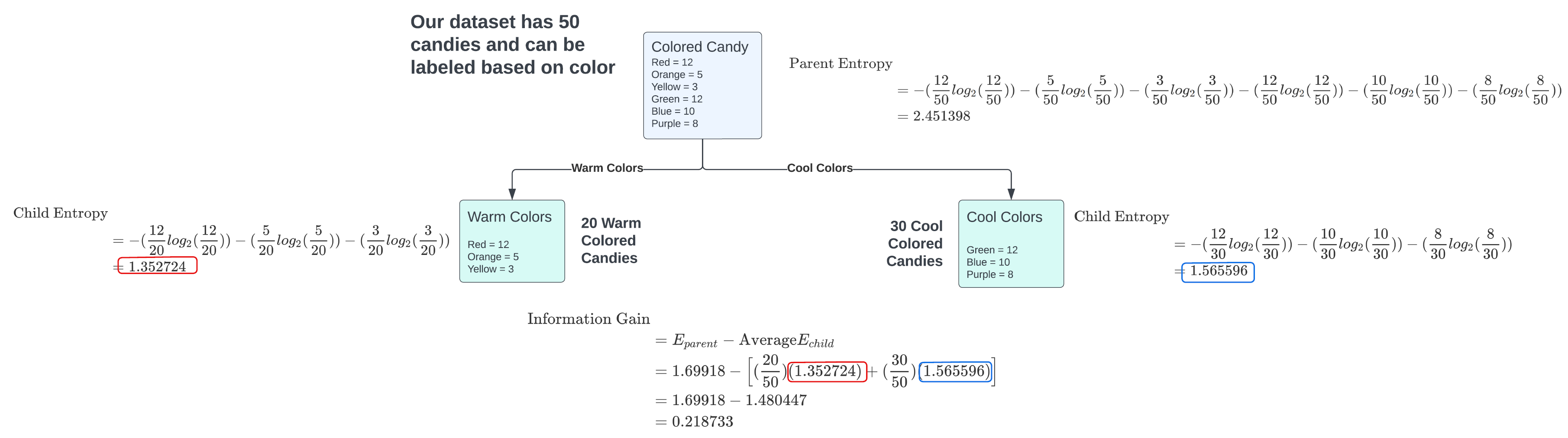
For the split on “warm colors” vs “cool colors” the colored candy’s decision tree split had an information gain of 0.218733. One could perform any kind of split on the colored candy’s and by following the same steps above then comparing this new split with the one shown above will show which is a more effective split for the colored candy dataset.
Creating an Infinite Number of Trees
Creating decision trees can lead to infinite variations, especially when handling continuous numerical data. This is because decision trees are adaptable and can be quite sensitive to changes in data and variables. One of the reasons for this variability is the challenge presented by continuous variables. The decision tree algorithm needs to decide where to split these variables into branches. Since there are countless potential split points within a continuous variable’s range, different decision trees can emerge.
Data variability also plays a role in generating different trees. Even small changes in the dataset or the order of data points can result in different splits and, consequently, different decision trees. This effect is more noticeable when working with large datasets with many features. The depth and complexity of decision trees also contribute to this diversity. Deeper trees can capture intricate data patterns but may overfit, while shallower ones might underfit. Thus, choices about the tree’s depth and complexity can lead to varying decision trees.
To address this challenge, use techniques like pruning, ensemble methods (e.g., Random Forests, Gradient Boosting), and cross-validation. These methods enhance the reliability and generalization of decision trees in practical applications.
Model Evaluation Metrics
A confusion matrix is a fundamental tool in machine learning that provides a comprehensive assessment of the performance of a classification model. It is particularly useful for evaluating the effectiveness of decision trees, a popular algorithm in this field.
A confusion matrix categorizes the model’s predictions into four key metrics: true positives (correctly predicted positive instances), true negatives (correctly predicted negative instances), false positives (incorrectly predicted positive instances), and false negatives (incorrectly predicted negative instances). These metrics help assess the model’s ability to distinguish between different classes.
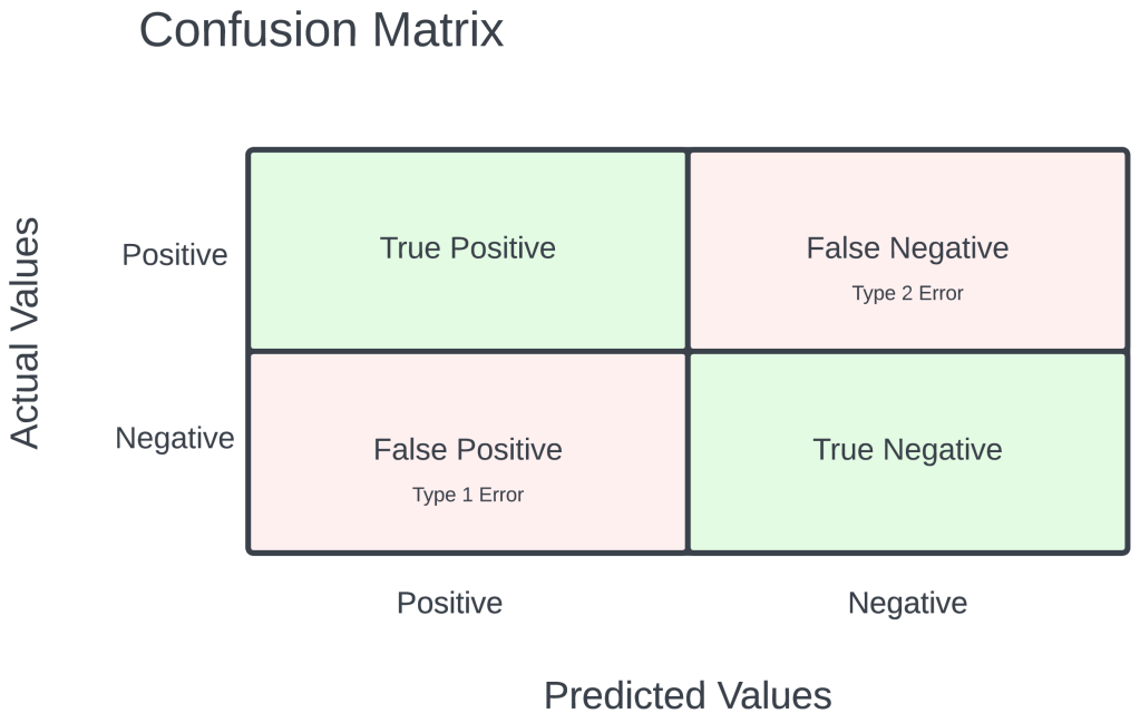
In the context of decision trees, accuracy is a crucial evaluation metric. It represents the ratio of correct predictions (sum of true positives and true negatives) to the total number of instances in the dataset. High accuracy indicates that the decision tree model is making accurate predictions, while a low accuracy suggests that the model is making numerous errors in classifying data points. However, accuracy alone might not provide a complete picture of a model’s performance, so it’s important to consider other metrics, such as precision, recall, and F1-score, in conjunction with the confusion matrix to gain a more nuanced understanding of the model’s capabilities.
Data Prep
For the analysis of Wildfires in the United States from 2000 to 2022, the decision tree modeling was performed on multiple datasets each with different purposes of them. These include quantitative values for the Acres Burned identifying the time of year the fire took place to that of predicting the topic of an article based on the words used its headline. In order to perform supervised learning appropriately each of the datasets were split into disjoint training and testing datasets with their labels removed (but kept for reference and accuracy analysis). In supervised learning, labels are essential for two primary reasons. They provide the correct output for a given input, allowing the algorithm to learn and make predictions. Labels also enable model evaluation and performance assessment, serving as the basis for key metrics.
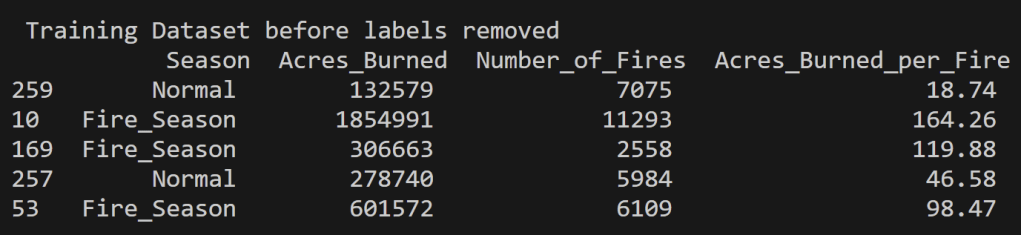
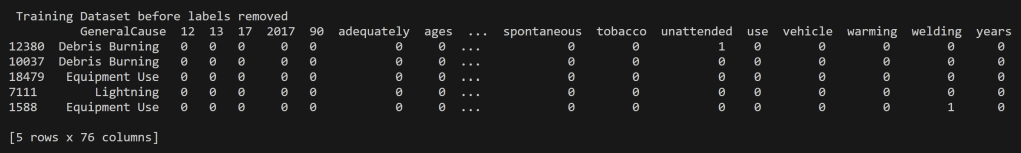
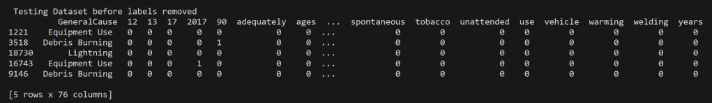
Below is the training and testing datasets that used a random split to have 80% of the data for training and 20% for testing. The goal for a good training set is for all of the possible data values to be represented and be represented in a proportion such that overfitting/underfitting for particular values doesn’t occur. All cleaned data used in this analysis can be found in the project GitHub repository here. Note that the datasets below have the labels still attached for reference, but they were removed from the testing set when running the predictions using the decision tree model.
US Wildfires By Season for Years 2000 to 2022

News Headlines from September 16th, 2023
News Headlines for topics “wildfire” and “weather” from September 16th, 2023
Oregon Weather and Wildfires Cause Comments Years 2000 to 2022
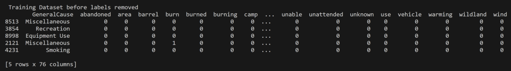

Oregon Weather and Wildfires Specific Cause Comments Years 2000 to 2022
Why Disjoint Training and Testing Data Sets
In machine learning, it is important to have training and testing data disjoint for several reasons, which are related to the goals of building a reliable model. Disjoint training and testing data help ensure that the model can effectively learn patterns from data and make accurate predictions on unseen, real-world examples. Testing on the training data does not prove that the model works on new data, new data is required to prove that, thus a disjoint testing set. Testing data is used to evaluate the performance of the model. It acts as a tool for how well the model will perform on new, unseen data. By keeping the testing data separate from the training data, one can assess how well the model generalizes to unseen instances. If one uses the same data for both training and testing, your model may simply memorize the training data rather than learning general patterns. This can lead to overfitting, where the model performs well on the training data but poorly on new data. Disjoint data prevents data leakage, ensuring that the model does not inadvertently learn from the testing data.
In many real-world applications, machine learning models are used to make important decisions. Disjoint testing data provides a higher level of trust and credibility in the model’s performance, which is essential for applications like medical diagnosis, autonomous driving, and financial predictions. To implement this separation, it is common practice to split the dataset into three parts: training data, validation data (used for model tuning if necessary), and testing data. The exact split ratio may vary depending on the size of your dataset, but the key idea is to ensure that the data used for testing is completely independent of the data used for training. For the supervised learning technique, only a training and testing dataset split will occur. This is partly for simplicity, though for future analyses validation instills a more credible model.
Code
All code associated with the decision tree and for all other project code can be found in the GitHub repository located here. Also the specific decision tree code is in the file named decision_trees.py . Another note, some inspiration for the code is from Dr. Ami Gates Decision Trees in Python7 and from the sklearn library documentation.
Results
One of the hypotheses for this Wildfires in the United States exploration was that there is a “Fire Season”. During Exploratory Data Analysis Graphing it was noted that the months June, July, August, and September faced the most Acres Burned and the Most Number of Fires in the United States over the years 2000 to 2022. These months also had the most spread in their distributions of their acres burned. Thus, for the machine learning model of decision trees it was decided to create a model that labels months June through September as “Fire Season” and all other months as “Normal”. Then with this new label using the quantitative values of “Acres Burned”, “Acres Burned per Fire”, and “Number of Fires” as a method to determine if a row of data should be labeled as “Fire Season” or “Normal”. Below is the results of decision tree model using the Gini Index as the criterion for best split.
US Wildfires By Season for Years 2000 to 2022
Using the Months June, July, August, and September as “Fire Season” and all other months as “Normal”.
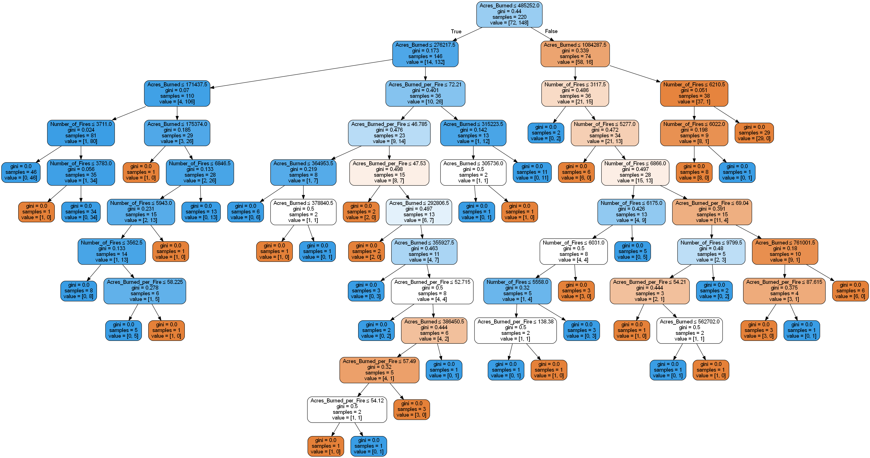

Accuracy = 80.35714285714286 %
Using Gini as the criterion one can see the results of the US wildfires “fire season” decision tree. This two class problem’s results show that it is indeed possible to model a “Fire Season” compared to “Normal” for the quantitative values associated with fires in the US. This model helps predict if a set of values (“Acres Burned”, “Acres Burned per Fire”, and “Number of Fires”) can be used to predict if the fire occurred in the months June through September.
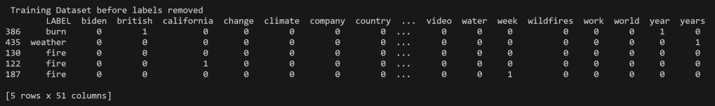
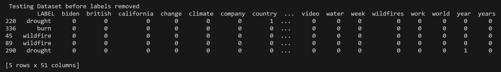
News Headlines for Wildfires, Burn, Fire, and Weather
News Headlines gathered on September 16th 2023 that contained topic words of “wildfire”, “burn”, “drought”, “fire”, and “weather”
Accuracy = 25%
Using Gini Values as the criterion, a decision tree model was constructed for the New Headlines Vectorized Data collected on September 16th, 2023. This dataset produced a notably intricate tree, indicating a high probability of overfitting. The results from the Confusion Matrix and the Accuracy clearly indicate that the model’s performance on the test data was subpar. Ideally, the diagonal squares should have exhibited the highest values, but this was not the case. The topic “fire” was frequently misclassified as “burn” in the headlines. This issue likely stems from the inherent similarity between headlines that pertain to these topics. It’s reasonable to assume that an article discussing a fire would also touch upon subjects that have been burned.
In an effort to address the challenge of dealing with words that have closely related contexts, a decision was made to streamline the topics to “wildfires” and “weather.” This decision aimed to simplify the model and minimize errors in the confusion matrix. The rationale behind this choice stemmed from prior analysis of the data, which revealed that the weather data predominantly centered around the discussion of the Hilary Hurricane in California, while the wildfire data focused on the Maui Fire.
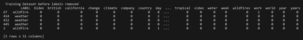
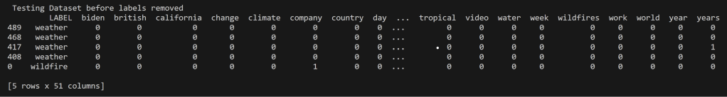
News Headlines for Wildfire and Weather
News Headlines gathered on September 16th 2023 that contained topic words of “wildfire” and “weather”
Accuracy = 85%
After reducing to a two class system we can see that the tree did become less complex and the confusion matrix and accuracy show way better results for how it performed on the test data. There was a 240% increase in the accuracy by changing the model to a two class problem. “weather” and “wildfire” were predicted accurately more than not.
Since headlines are always changing, this model is still plagued by a situation of overfitting for the day the headlines were pulled. The model might be mostly accurately predicting the labels of headlines from September 16th 2023, however, this does not demonstrate that it will accurately predict headline topics for say October 22nd 2023, or even September 16th 2000.
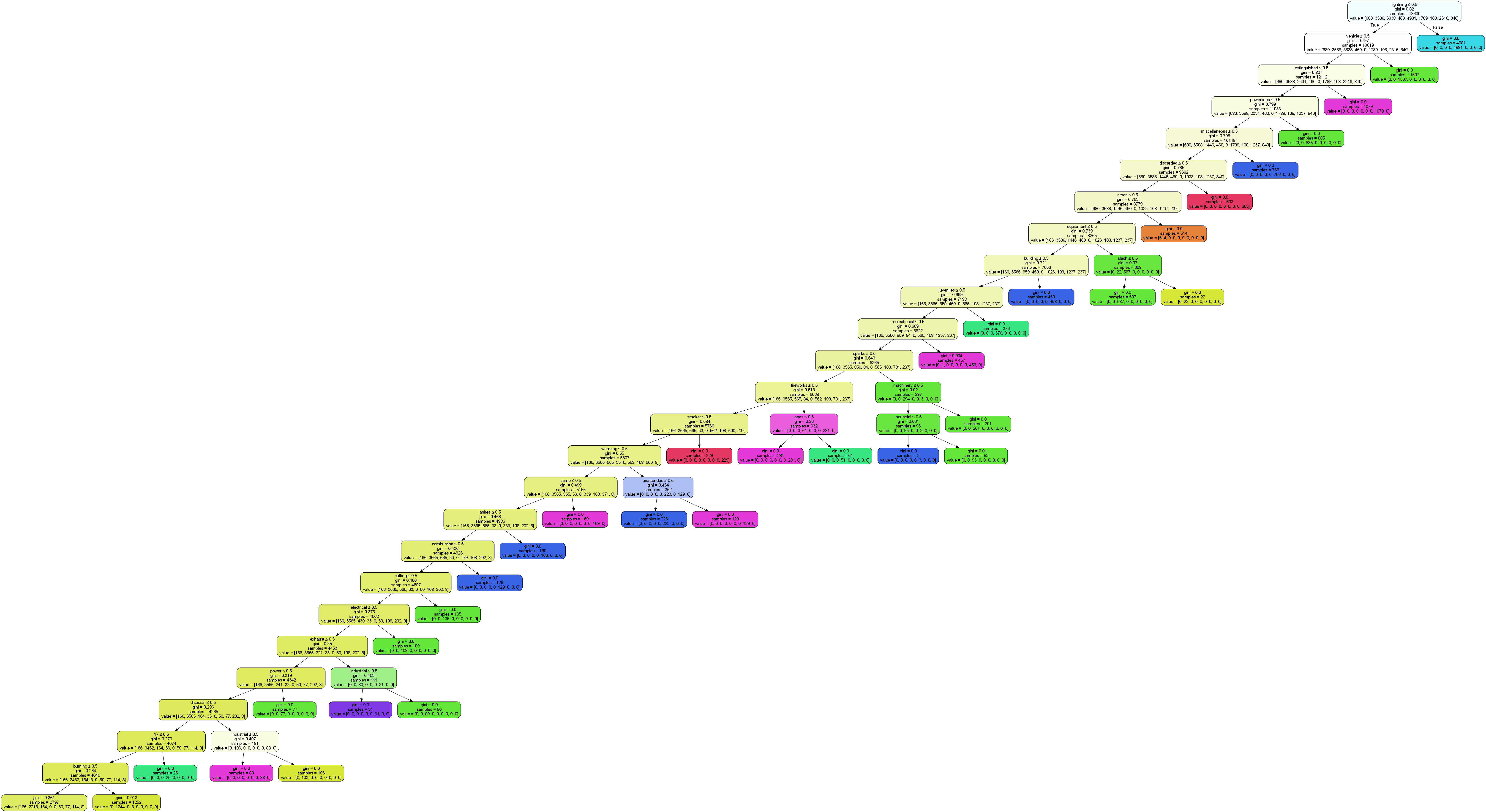
Oregon Weather and Wildfires Cause Comments
For the fire cause comment text data for fires in Oregon from the years 2000 to 2022.

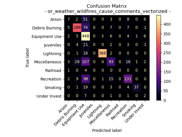
Accuracy = 71.0204081632653%
The above decision tree for the modeling of cause comments is extremely complex. It is important to note that this the above decision tree was limited by a maximum depth of 25. Meaning that not all of the terminal nodes are pure. With that in mind from the confusion matrix, the extremely complex model did a less than ideal job of accurately predicting the appropriate label for the test data. Some cause labels wear seen to be predicted well (as noted in the confusion matrix). These include “Debris Burning”, “Equipment Use”, and “Lighting”, but “Railroad” was never accurately predicted.
Oregon Weather and Wildfires Specific Cause Comments
For the fire cause comment text data for fires in Oregon from the years 2000 to 2022.
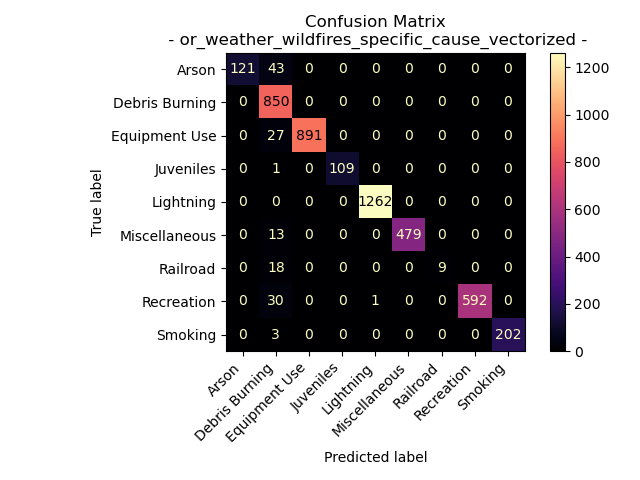
Accuracy = 97.07589765641798%
Interestingly the specific cause comment data from the Oregon Weather and Wildfire Data created a less complex decision tree (still with a max depth limit of 25) with a more accurate model as seen by the results of the confusion matrix. The labels for the cause comments and the specific comments are the same, but the text data used form each label is different. A possible theory as to why this data creates a better model is that specific cause comments might be more unique to each label, making them more distinct when splitting.
Another note is that both models did a great job of predicting “Lightning”, “Debris Burning”, and “Equipment Use”. Especially “Lightning” as one can see the specific cause model accurately predicted lighting as the cause 99.9% of the time. Moving forward it would be wise to use the specific cause comments decision tree model for evaluating the general cause of the fire over that of the cause comments.
Conclusions
For US wildfires from 2000 to 2022, the analysis initially explored the concept of a “Fire Season,” which was observed to primarily occur during the months of June through September, characterized by the highest occurrences of Acres Burned and Number of Fires. We developed a decision tree model to classify months as either “Fire Season” or “Normal,” based on quantitative metrics like “Acres Burned,” “Acres Burned per Fire,” and “Number of Fires.” The results using the Gini Index as the criterion revealed an accuracy of 80.36%, suggesting the viability of modeling a “Fire Season” based on these quantitative values.
In contrast, the application of decision trees to New Headlines Vectorized Data collected on September 16th, 2023, exhibited a more complex tree structure and an accuracy of only 25%. This model’s poor performance on the test data, as evidenced by the Confusion Matrix, was largely attributed to the overlapping context of words like “wildfire” and “burn” in headlines. This complexity was mitigated by simplifying the model into two primary topics, “wildfire” and “weather,” yielding a significantly improved accuracy of 85% The decision to streamline these topics was motivated by prior data analysis, which revealed a clearer distinction between the two.
However, it’s essential to recognize that the machine learning models, despite their accuracy, are sensitive to the specific data and date of collection. While the models may perform well for headlines from September 16th, 2023, their adaptability to different dates or years remains uncertain.
Additionally, the analysis extended to Oregon Weather and Wildfires Cause Comments and Specific Comments. The former yielded a highly complex decision tree with varying levels of accuracy for different cause labels. In contrast, the Specific Comments data led to a less complex decision tree with an impressive accuracy of 97.08%. This suggests that specific cause comments are more distinctive and result in a more accurate model, with “Lightning,” “Debris Burning,” and “Equipment Use” emerging as particularly well-predicted causes.
Moving forward, it is prudent to use the decision tree model based on specific cause comments for evaluating the general cause of wildfires, as it demonstrated a more robust performance. Nonetheless, it’s essential to acknowledge that the effectiveness of these models may vary depending on the nature of the data and the specific context of their application.
- IBM. “What Is a Decision Tree | IBM.” Www.ibm.com, www.ibm.com/topics/decision-trees#:~:text=A%20decision%20tree%20is%20a. ↩︎
- Raturi, Akriti. “What’s a Decision Tree and Its Application? – Igebra.” Igebra.ai, 13 June 2023, www.igebra.ai/blog/whats-a-decision-tree-and-its-application/. Accessed 18 Oct. 2023. ↩︎
- IBM. “What Is a Decision Tree | IBM.” Www.ibm.com, www.ibm.com/topics/decision-trees#:~:text=A%20decision%20tree%20is%20a. ↩︎
- Nagesh Singh Chauhan. “Decision Tree Algorithm, Explained – KDnuggets.” KDnuggets, 9 Feb. 2020, www.kdnuggets.com/2020/01/decision-tree-algorithm-explained.html. ↩︎
- Dash, Shailey. “Decision Trees Explained — Entropy, Information Gain, Gini Index, CCP Pruning..” Medium, 2 Nov. 2022, towardsdatascience.com/decision-trees-explained-entropy-information-gain-gini-index-ccp-pruning-4d78070db36c#:~:text=In%20the%20context%20of%20Decision. ↩︎
- Dash, Shailey. “Decision Trees Explained — Entropy, Information Gain, Gini Index, CCP Pruning..” Medium, 2 Nov. 2022, towardsdatascience.com/decision-trees-explained-entropy-information-gain-gini-index-ccp-pruning-4d78070db36c#:~:text=In%20the%20context%20of%20Decision. ↩︎
- Gates, Ami. “Decision Trees in Python – Gates Bolton Analytics.” Gates Bolton Analytics, gatesboltonanalytics.com/?page_id=282. Accessed 20 Oct. 2023. ↩︎
